Score-Based Allocation
Allocation distributes limited supply across competing demands using a deterministic, score-based priority system. It runs after the supply pipeline step (auto-triggered) or standalone via CLI/API, over a 13-week default horizon (one fiscal quarter).
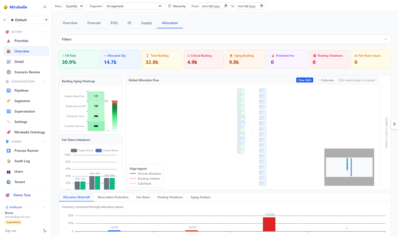
Table of Contents
- Overview
- Core Concepts
- The 8-Pass Algorithm
- Policy Layers
- Allocation Tab in Dashboard
- Detail View
- Time-Phased Allocation Timeline
- Troubleshooting — "Requested 0, Allocated 0, Score 6000"
- Explainability
- Running Allocation
- Configuration
Overview
When demand exceeds supply, not every order can be fulfilled. Allocation answers the question: which demands get the available stock, and how much?
Mirabelle's allocation engine solves this by assigning every demand a composite score derived from business rules (priority class, strategic value, urgency, fairness), then allocating supply greedily from the highest-scored demand downward. The result is a deterministic, auditable, and explainable assignment of inventory to orders.
When does it run?
| Trigger | Description |
|---|---|
| Auto (pipeline) | After the supply step completes, allocation runs automatically on the netted forecast and planned supply |
| Manual (API) | POST /api/allocation/run |
| Manual (CLI) | python -m files.run_pipeline --only allocation |
13-week horizon
The default horizon is 13 weeks (one quarter). Beyond 13 weeks the candidate cardinality grows prohibitively large for typical datasets. Override with the ALLOCATION_HORIZON_WEEKS environment variable.
Core Concepts
Demands
Each demand represents a single (item, site, week) combination requiring supply:
| Source | Table | Description |
|---|---|---|
| Unconsumed forecast | PIPE_forecast_netting |
Net demand after netting (statistical + maintenance minus returns, minus firm order consumption) |
| Firm future orders | master.demand_actuals |
Confirmed customer orders where is_forecast = false and date falls within the horizon |
The netting step (see Supply Planning > Netting) already combines unconsumed forecast with firm demand into supply_plan_qty. Allocation consumes this final figure.
Supplies
Each supply record represents inventory or planned orders available to fulfil demands:
| Source | Table | Details |
|---|---|---|
| On-hand inventory | master.on_hand |
Aggregated per (item, site, type) where planning_type IN ('good', 'new') |
| Planned supply orders | PIPE_supply_orders |
Status in ('planned', 'firm', 'released', 'in_transit') — purchase, transfer, make, or repair orders |
Allocation Unit
One demand is one (item, site, week) tuple. The engine never splits a single demand across multiple supply sources for the same week—though partial fulfilment is allowed when total supply is insufficient.
Composite Score
Every eligible (demand, supply) pair receives a composite score:
total_score = priority + aging + lateness
            + strategic + revenue + criticality
            − routing_penalty − fairness_penalty − reservation_penalty
Higher total scores are allocated first. The score breakdown is stored per allocation and is fully explainable (see Explainability).
The 8-Pass Algorithm
The allocation engine (implemented in Rust for performance) executes eight deterministic passes:
flowchart LR
    A[1. Enrich] --> B[2. Seed Fairness]
    B --> C[3. Build Reservations]
    C --> D[4. Generate Candidates]
    D --> E[5. Filter Hard Constraints]
    E --> F[6. Score Candidates]
    F --> G[7. Sort by Score]
G --> H[8. Greedy Allocation]| Pass | Name | What happens |
|---|---|---|
| 1 | Enrich backlog | Compute backlog_days = current_date − required_date for each demand; attach priority class, strategic/revenue/criticality weights from master.item |
| 2 | Seed fairness tracker | Register each demand's group (channel, customer class, or program) and quantity into the fairness state machine |
| 3 | Build reservations | Reservation engine fences a portion of each supply for high-priority future demands (e.g. AOG orders arriving within the lookahead window) |
| 4 | Generate candidates | Create (demand, supply) pairs where item_id and location_id match, and supply arrives within the demand's max-delay tolerance |
| 5 | Filter hard constraints | Remove candidates that violate hard routing rules (e.g. supply location not in the allowed set). These candidates are permanently excluded |
| 6 | Score candidates | Compute the composite score for every remaining candidate in parallel (Rayon). Positive components: priority, aging, lateness, strategic, revenue, criticality. Negative penalties: routing soft violations, fairness over-share, reservation trespass |
| 7 | Sort descending | Sort all scored candidates by total_score DESC, with deterministic tiebreak on (demand_id, supply_id) |
| 8 | Greedy allocation | Walk the sorted list. For each candidate: check remaining supply (minus reservation fences), check remaining demand, check fairness hard cap. Allocate min(demand_remaining, supply_remaining). Update trackers. Continue until all candidates are exhausted |
Determinism
The same inputs always produce the same outputs, including tiebreaks. Re-running allocation with unchanged data yields identical results.
Policy Layers
Seven policy types control allocation behaviour. Each is stored as a parameter set in the database and resolved per scenario (with optional segment-level overrides).
Priority
The priority policy defines the base score each priority class receives and the multipliers applied to business weights:
| Priority Class | Default Score | Typical Use |
|---|---|---|
| AOG | 10 000 | Aircraft-on-ground / emergency — must ship immediately |
| Critical | 5 000 | Key customer commitments, contractual SLAs |
| Premium | 2 000 | High-value orders, strategic accounts |
| Standard | 1 000 | Normal business demand |
| Low | 100 | Fill-in orders, low-margin SKUs |
Three global weight factors scale the business-weight components:
| Factor | Affects | Default |
|---|---|---|
strategic_weight_factor |
demand.strategic_weight × factor |
1.0 |
revenue_weight_factor |
demand.revenue_weight × factor |
1.0 |
criticality_weight_factor |
demand.criticality_weight × factor |
1.0 |
Effect on allocation
Increasing a weight factor amplifies the differentiation between items that have different master.item weight values. If all items have weight = 0, changing the factor has no effect.
Starvation
The starvation policy prevents low-priority demands from receiving zero allocation indefinitely.
| Parameter | Default | Meaning |
|---|---|---|
enabled |
true |
Activate anti-starvation logic |
escalation_threshold_days |
14 | Days a demand must be overdue before escalation begins |
score_per_extra_day |
50 | Bonus points added per day beyond the threshold |
max_starvation_bonus |
3 000 | Cap on total starvation bonus (0 = uncapped) |
auto_upgrade_priority |
false |
Automatically bump the demand's PriorityClass by one level when threshold is crossed |
When a standard demand has been waiting 20 days past its required date, the starvation bonus is:
This can push a long-waiting standard demand above a fresh premium demand, ensuring it eventually gets served.
Reservation
The reservation policy fences a portion of supply for high-priority future demands.
| Parameter | Meaning |
|---|---|
enabled |
Activate reservation fences |
lookahead_days |
How far ahead to scan for protected demand (e.g. 7 days) |
min_protected_priority |
Minimum priority class to protect (e.g. AOG) |
penalty |
Score penalty applied to lower-priority candidates that attempt to consume reserved supply |
safety_margin |
Extra buffer percentage added to the reserved quantity |
Reservation in action
If 100 units are on hand and an AOG demand is expected in 5 days (within the 7-day lookahead), the reservation engine may fence 100 units. A low-priority demand today would face a penalty of 99 999 points for consuming that reserved supply—effectively blocking it and preserving the stock for the upcoming AOG order.
Figure: a reservation fence is scanned in within the lookahead window, subtracted from available supply, then either consumed by the protected demand or released when the window expires.
stateDiagram-v2
  [*] --> Scanning: lookahead window
  Scanning --> Fenced: protected demand found<br/>(qty x (1 + safety_margin))
  Fenced --> Reserved: fence subtracted from supply pool
  Reserved --> Consumed: higher-priority demand arrives
  Reserved --> Released: lookahead expires / no demand
  Consumed --> [*]
Released --> [*]Fairness
The fairness policy ensures no single channel, customer class, or program monopolises supply.
| Parameter | Meaning |
|---|---|
enabled |
Activate fairness tracking |
group_field |
Dimension for grouping: channel, customer_class, or program |
target_shares |
Map of group name → target share (e.g. {"A": 1.0, "B": 1.0} = 50/50) |
tolerance |
Acceptable deviation from target share (default 0.05 = ±5%) |
hard_cap |
If true, groups that exceed their share are hard-blocked from further allocation |
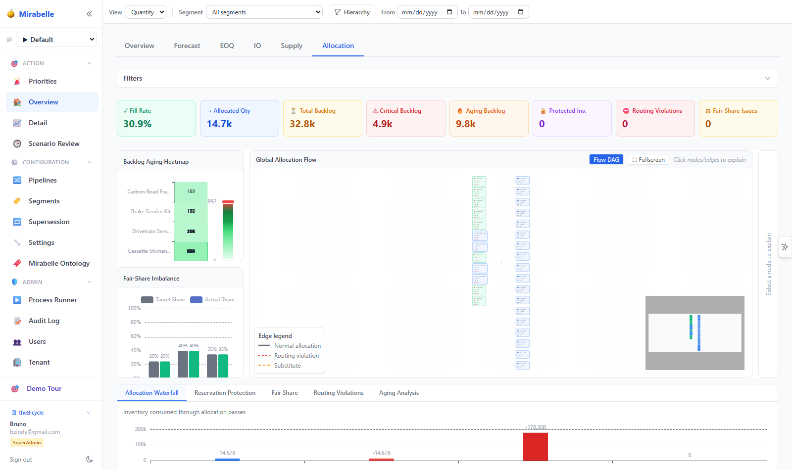
When fairness is active, the engine penalises candidates whose group is already above its target share, and (with hard_cap: true) can entirely block an over-served group from receiving more.
Routing
The routing policy validates that a supply source is compatible with a demand's fulfilment constraints.
| Mode | Effect |
|---|---|
| Hard | Candidate is removed if the supply location is not in the allowed_locations set, or if the supply's inventory_pool / routing_tags don't match the policy |
| Soft | Candidate remains eligible but receives a score penalty proportional to the violation severity |
Multiple routing policies can coexist (one per row in the parameter set), each keyed by policy_id. A demand references its routing policy via routing_policy_id.
Aging
The aging policy rewards older unfulfilled demands with a higher score, ensuring that demands don't languish forever behind newer high-priority orders.
| Mode | Formula | Use case |
|---|---|---|
| Linear | multiplier × backlog_days |
Steady urgency increase |
| Exponential | multiplier × backlog_days^exponent |
Rapidly escalating urgency for very old demands |
The aging component stacks with the starvation bonus (aging is the base, starvation adds on top when the threshold is crossed).
Lateness
The lateness curve defines how expected delivery delay translates into a score adjustment.
| Curve type | Behaviour |
|---|---|
| Linear | −penalty_rate × delay_days — proportional penalty for late fulfilment |
| Quadratic | −penalty_rate × delay_days² — sharply penalises very late fulfilments |
| Step | Fixed penalty above a threshold — binary on-time / late |
Lateness is scored relative to the supply's available date vs. the demand's required date. A demand paired with early supply gets no penalty; pairing with late supply incurs a penalty proportional to the delay.
Allocation Tab in Dashboard
The Allocation tab on the Dashboard (/) provides an aggregate view of the latest allocation run.
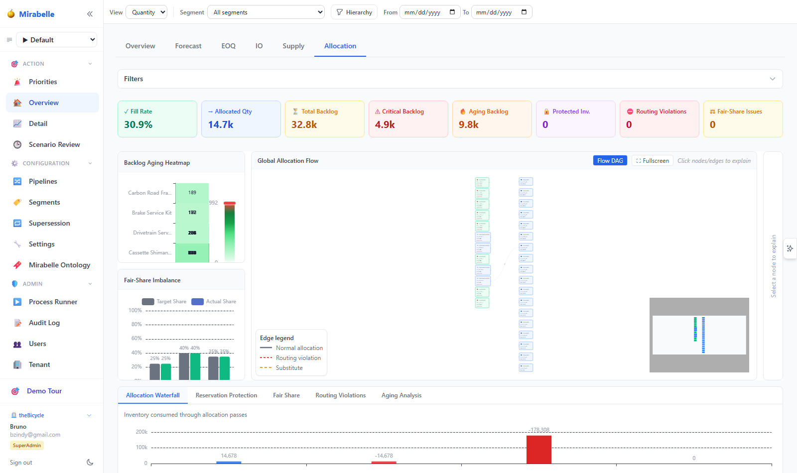
Figure: the Allocation tab fans the latest run out into KPI cards and visual panels — DAG, backlog heatmap, waterfall, fair-share, and aging distribution.
flowchart TD
  RUN["Latest allocation run"] --> K["KPI cards<br/>(fill rate, filled, unfulfilled)"]
  RUN --> DAG["Allocation DAG<br/>(demand-supply flow)"]
  RUN --> HM["Backlog heatmap<br/>(top-40 shortfalls)"]
  RUN --> WF["Waterfall chart<br/>(stock -> alloc -> shortage)"]
  RUN --> FS["Fair-share chart<br/>(actual vs target)"]
  RUN --> AG["Aging distribution<br/>(backlog days)"]
View Mode
All allocation panels respect the View Mode dropdown in the toolbar (Quantity / Cost / Price / Margin). When the view is set to a monetary mode:
- KPI cards show currency values instead of unit counts (e.g. "€25,400 backlog" instead of "59 units")
- Backlog heatmap cells display monetary value
- Waterfall chart steps are in currency
- Fair-share chart shows monetary allocation per group
- Reservation timeline bars show allocated/reserved/available in currency
- The DAG graph node sizes reflect monetary value
The conversion uses qty × avg_unit_cost (global average from master.item + master.item_location) followed by currency conversion via /api/currency-conversions. If avg_unit_cost is 0 or missing, all monetary-mode panels render as zero — this is the most common cause of "empty allocation charts in price/cost/margin mode."
KPI Cards
Figure: allocation KPIs branch from three roots — fill-rate ratio, demand disposition (full/partial/unfilled), and violation/inventory signals.
flowchart TD
  FR["Fill Rate"] --> FR1["total_allocated / total_demand"]
  D["Demands"] --> DF["Fully filled"]
  D --> DP["Partially filled"]
  D --> DU["Unfilled"]
  V["Violations"] --> VR["Routing"]
  V --> VF["Fair-share"]
  P["Protected inventory"] --> PR["reserved qty"]
L["Late demand count"] --> LU["remaining unfulfilled"]| Card | Meaning |
|---|---|
| Fill Rate | Total allocated ÷ total demanded (percentage) |
| Total Demands | Number of distinct demand IDs in the run |
| Filled | Demands that received 100% of requested quantity |
| Unfulfilled | Demands that received 0% of requested quantity |
| Routing Violations | Allocations where a soft routing constraint was violated |
| Fair-share Violations | Allocations where a fairness correction was applied |
| Protected Inventory | Quantity reserved by reservation fences |
| Late Demand Count | Demands with remaining unfulfilled quantity |
Visual Panels
| Panel | Description |
|---|---|
| Allocation DAG | Directed acyclic graph showing demand → supply → allocation flows. Node size = quantity. Colour = priority class |
| Backlog Heatmap | Top-40 item/site pairs by shortfall, colour-coded by severity |
| Waterfall Chart | Starting stock → allocations → shortages → remaining stock |
| Fair-share Chart | Actual vs. target share per fairness group |
| Routing Violations Table | List of allocations with soft routing violations, including supply ID and penalty magnitude |
| Aging Distribution | Histogram of unfulfilled demands by backlog days |
Detail View
Click any item/site row to drill into the Allocation Detail view.
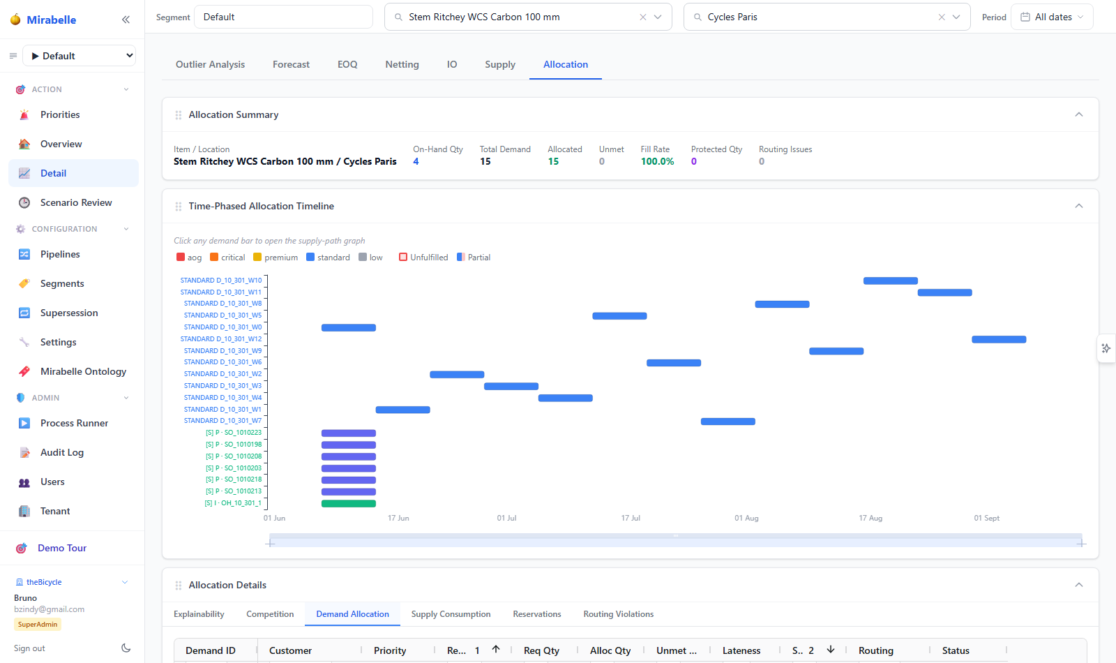
Header KPIs
| KPI | Source |
|---|---|
| Item & Site names | master.item, master.site |
| On-hand quantity | master.on_hand (all pools) |
| Total demand | Sum of all demands for this (item, site) |
| Allocated | Sum of allocated quantity |
| Unmet | Sum of shortfall quantity |
| Protected | Quantity held by reservations |
| Routing violations | Count of allocations with routing penalty > 0 |
Time-Phased Allocation Timeline
The Time-Phased Allocation Timeline is a Gantt-style chart (AllocationTimeline.jsx) that shows, for the selected part (item_id + site_id), how each demand week was matched against available supply.
Layout
| Row band | What it shows |
|---|---|
Bottom rows [S] |
Supply buckets — on-hand inventory (OH_…), purchase orders, transfers, repairs. Each bar is one week wide, positioned at the supply's available_date. Colour by source type (green = inventory, indigo = purchase order, violet = manufacturing, amber = transfer, pink = repair). |
| Top rows | Demand weeks. The demand_id is built as D_{item_id}_{site_id}_W{week_index} (e.g. D_14_303_W6), so one bar appears per forecast week in the horizon. Colour by priority class (red = AOG, orange = critical, yellow = premium, blue = standard, grey = low). |
Bar styling encodes fulfilment status:
| Style | Meaning |
|---|---|
| Solid fill | Fully allocated (status = full) |
| Right-edge stripe | Partial allocation (status = partial) |
| Dashed red outline + faded fill | Unfulfilled (status = unfulfilled) |
| Solid red border | Late fulfilment (lateness_days > 0) |
Purple dashed vertical lines mark reservation fences (supply held back for future high-priority demand).
Hover tooltip
Hovering a demand bar shows:
| Field | Meaning |
|---|---|
| Demand ID | D_{item}_{site}_W{n} |
| Priority | AOG / Critical / Premium / Standard / Low |
| Status | full / partial / unfulfilled |
| Requested | Total quantity demanded that week |
| Allocated | Quantity actually satisfied |
| Score | Composite allocation score (see below) |
| ⏱ late | Days late, if the supply arrives after the required date |
Click → Supply Path
Clicking a demand bar selects it and opens the Supply Path Modal (see below), which traces the complete demand → supply → source chain for that single week. Clicking a supply bar selects that supply in the consumption table.
How the numbers are computed
The chart is fed by GET /api/allocation/detail/{item_id}/{site_id}/timeline. For each demand week it aggregates, in ClickHouse, the PIPE_allocation_results rows grouped by demand_id:
SELECT demand_id, sum(allocated_qty), sum(total_score)
FROM PIPE_allocation_results
WHERE pipeline_id = … AND scenario_id = … AND archive_date = … AND run_id = …
  AND item_id = {item} AND site_id = {site}
GROUP BY demand_id ORDER BY sum(allocated_qty) DESC LIMIT 18
It then reconciles against PIPE_allocation_unfulfilled:
- Demand is in the unfulfilled table →
requested = requested_qty + allocated_qty,allocated = allocated_qty, status =unfulfilledorpartial - Demand is NOT in the unfulfilled table → treated as fully filled:
requested = allocated = sum(allocated_qty), status =full
The Score field
Score is sum(total_score) — the composite allocation priority the Rust engine computed per (demand, supply) candidate, summed across every supply that fed that demand week:
total_score = priority + aging + lateness
            + strategic + revenue + criticality
            − routing_penalty − fairness_penalty − reservation_penalty
The score is independent of quantity — it reflects priority and business weights, not how much was committed. With default allocation_priority settings, standard = 1 000, critical = 5 000, aog = 10 000 (see Policy Layers › Priority). A score of 6 000 on a standard demand typically means 6 supply candidates were scored for that week (6 × 1 000), or a mix of priority + aging components.
Troubleshooting — "Requested 0, Allocated 0, Score 6000"
If every bar shows Requested 0, Allocated 0 but a non-zero Score, two things are true at once:
- Bars render → there are
PIPE_allocation_resultsrows for this (item, site) — the empty-state guard did not trigger, so the run produced scored candidate rows. - Requested/Allocated = 0 →
sum(allocated_qty)perdemand_idrounds to 0, and there is no matching row inPIPE_allocation_unfulfilled. The endpoint then takes the fallback branch whererequested = allocated ≈ 0and (incorrectly) labels the status"full".
The non-zero Score is the unrounded sum(total_score): the engine scored demand for this part against available supply, but committed ~0 quantity to it (supply exhausted by higher-priority demands, or near-zero supply_plan_qty).
Diagnose with these ClickHouse queries
Replace :pid, :sid, :ad with the active pipeline / scenario / archive_date (the same values the page uses — visible in the URL query string):
-- 1. What's actually stored for this part's allocation rows
SELECT demand_id, supply_id, allocated_qty, total_score, score_priority
FROM PIPE_allocation_results
WHERE pipeline_id = :pid AND scenario_id = :sid AND archive_date = :ad
  AND item_id = 14 AND site_id = 303
ORDER BY demand_id, total_score DESC;

-- 2. Are there shortfall / unfulfilled rows for it?
SELECT demand_id, requested_qty, allocated_qty, shortfall_qty, arrayJoin(reasons)
FROM PIPE_allocation_unfulfilled
WHERE pipeline_id = :pid AND scenario_id = :sid AND archive_date = :ad
  AND item_id = 14 AND site_id = 303;

-- 3. The demand qty that was fed in (should be > 0)
SELECT item_id, site_id, forecast_week, supply_plan_qty
FROM PIPE_forecast_netting
WHERE pipeline_id = :pid AND scenario_id = :sid AND archive_date = :ad
  AND item_id = 14 AND site_id = 303 AND supply_plan_qty > 0
ORDER BY forecast_week;

-- 4. The supply that was available to satisfy it
SELECT supply_id, source_type, qty_available, available_date
FROM PIPE_supply_orders
WHERE pipeline_id = :pid AND scenario_id = :sid AND archive_date = :ad
  AND item_id = 14 AND site_id = 303;
Query 1 reveals whether allocated_qty is genuinely tiny (rounding to 0) or exactly 0. Query 2 confirms whether the missing-unfulfilled-row path is why requested collapses to 0. If query 2 is empty while query 1 has zero-qty rows, those demands should have been written to PIPE_allocation_unfulfilled — the shortfall rows were dropped during write_results_ch().
Demo — competition scenarios on /series/14_303
A seeded demo on item 14 / site 303 (pipeline 4) makes the timeline a meaningful competition showcase. It is set up by files/scripts/seed_alloc_demo_14_303.py (idempotent; --restore undoes it).
What was wrong before: the seeded demand for 14_303 was ~0.4 units/week (sub-unit → rounded to 0 in the tooltip), no firm orders → no customer, and supply far exceeded demand → nothing competed.
The demo seed creates 13 weekly firm orders (160 units total) attached to named customers with mixed priority classes, against ~117 units of available supply (50 on-hand + 67 planned):
| Week | Qty | Customer | Priority | Outcome |
|---|---|---|---|---|
| W2 | 25 | UAE Team Emirates | AOG (10 000) | ✅ full |
| W4 | 18 | Visma-Lease a Bike | critical (5 000) | ✅ full |
| W0 | 15 | Ineos Grenadiers | premium (2 000) | ✅ full |
| W6 | 14 | Ineos Grenadiers | premium (2 000) | ✅ full |
| W1 | 10 | Berlin Cycling Club | standard (1 000) | ✅ full |
| W10 | 11 | Équipe Amateurs Tour | standard (1 000) | ✅ full |
| W12 | 16 | Berlin Cycling Club | standard (1 000) | ◐ partial (9/16) |
| W3 | 8 | Barcelona Riders Club | standard | ❌ unfulfilled |
| W5 | 10 | Équipe Amateurs Tour | standard | ❌ unfulfilled |
| W8 | 12 | Berlin Cycling Club | standard | ❌ unfulfilled |
| W7 | 8 | Barcelona Riders Club | low (100) | ❌ unfulfilled |
| W9 | 7 | Barcelona Riders Club | low | ❌ unfulfilled |
| W11 | 6 | Barcelona Riders Club | low | ❌ unfulfilled |
The story for a demo: with demand (160) exceeding supply (117), the engine rations by composite score. AOG and critical orders consume the on-hand pool first; premium orders follow; standard orders split the remainder (some full, one partial); and the low-priority amateur orders plus the late standard orders receive nothing — visible as dashed-red unfulfilled bars. Hover any bar to see the customer name, priority class, requested vs allocated, and the composite score.
Re-running the demo (after editing the seed quantities or to refresh after a forecast re-run):
python files/scripts/seed_alloc_demo_14_303.py            # seed firm orders + on-hand
python -m files.run_pipeline --only netting    --pipeline-id 4 --scenario-id 4
python files/scripts/seed_alloc_demo_14_303.py --restore   # undo
Netting must be re-run so the firm orders flow into PIPE_forecast_netting.supply_plan_qty (= unconsumed forecast + firm demand), which is what allocation consumes. Allocation is then re-run from the series page (it reads the latest run for the pipeline's supply_scenario_id).
Two bugs fixed to make the demo work
- Customer never shown — the timeline/demands/graph endpoints hardcoded
"customer": ""and"priority_class": "standard". They now look up the firm-order customer name + per-week priority frommaster.demand_actuals(is_forecast=false), matched by week-index (files/api/main.py: _alloc_firm_meta_by_week). - Firm-order priority never reached the scores —
load_demandssnapped firm-order dates to Monday-of-week, but this tenant's forecast weeks start on Sunday, so the firm-meta key never matched the nettingforecast_weekand every demand fell back tostandard. Fixed by keying firm-meta on the week-index ((date - planning_today).days // 7), which is convention-independent (files/allocation_runner.py: load_demands).
Supply Path Modal
Clicking a demand bar in the Time-Phased Allocation timeline or a row in the Demand Allocation table opens a centered overlay that shows the complete supply path for that single demand.

The modal lays out the chain left-to-right in three columns:
| Column | What it shows |
|---|---|
| Source (left) | Upstream origin: SOURCE WAREHOUSE (TRANSFER), Supplier (PURCHASE_ORDER), Production Line (MANUFACTURING), Repair Pool (REPAIR). No node for INVENTORY since on-hand IS the source. |
| Supply (middle) | One node per allocated supply. Each shows supply_id, source type, allocated qty, available qty, arrival/release weeks, and ERP status. Firm supplies carry a 🔒 FIRM badge. |
| Demand (right) | The demand node with priority class, item name, requested vs allocated qty. |
Edges carry the quantity flowing through them and the lead time for upstream legs.
The right-hand side panel summarises the demand, lists each contributing allocation (with the firm/recommendation share visualised), and remains in sync as you pan or zoom the graph. Close with the × button or the Esc key.
Demands Table
| Column | Description |
|---|---|
| Demand ID | Unique identifier (e.g. D_123_45_W6) |
| Priority Class | AOG / Critical / Premium / Standard / Low |
| Required Date | Week the demand is due |
| Requested Qty | Total quantity demanded |
| Allocated Qty | Quantity satisfied |
| Unallocated Qty | Remaining shortfall |
| Score | Composite score of the winning allocation |
| Score Breakdown | Expandable: priority, aging, lateness, strategic, revenue, criticality, penalties |
| Status | full / partial / unfulfilled |
| Flags | Routing violation, fairness-adjusted, reservation-blocked |
Supplies Table
| Column | Description |
|---|---|
| Supply ID | OH_ prefix = on-hand; SO_ prefix = supply order |
| Source Type | inventory / purchase_order / make / transfer / repair |
| Available Date | When the supply becomes usable |
| Qty Available | Total quantity |
| Qty Allocated | Quantity consumed by allocations |
| Qty Reserved | Quantity held by reservation fences |
| Qty Remaining | Unallocated surplus |
| Utilization | Allocated ÷ Available (percentage) |
| Consuming Demands | List of demand IDs fed by this supply |
Reservations
If the reservation policy is active, this panel shows:
- Reservation type (e.g.
future_premium) - Protected quantity
- Lookahead horizon (days)
- Protected priority classes (e.g. premium, aog)
- Reason text
Competition View
Select a supply ID to see which demands compete for it. The competition panel lists all demands paired with that supply, sorted by composite score descending, showing:
- Demand ID and priority class
- Requested and allocated quantity
- Composite score and full breakdown
- Routing / fairness / reservation flags
This is the key tool for answering: "Why did demand X lose to demand Y?"
Explainability
Every allocation (or unfulfilled demand) has a human-readable explanation. The explain endpoint returns a structured narrative describing exactly how the score was computed and which policies influenced the outcome.
API
Response Structure
{
  "demand_id": "D_123_45_W3",
  "priority_class": "STANDARD",
  "requested_qty": 200,
  "allocated_qty": 150,
  "unallocated_qty": 50,
  "status": "partial",
  "score": 1847.3,
  "score_breakdown": {
    "priority_component":    1000.0,
    "aging_component":       320.0,
    "lateness_component":    0.0,
    "strategic_component":   250.0,
    "revenue_component":    277.3,
    "criticality_component": 0.0,
    "routing_penalty":       0.0,
    "fairness_penalty":     -50.0,
    "reservation_penalty":   0.0
  },
  "allocation_narrative": [
    "Demand 'D_123_45_W3' (STANDARD) allocated 150.000 units from supply 'OH_123_45_2' at location '45'",
    "Score: 1847.30 = priority(1000.0) + aging(320.0) + lateness(0.0) + strategic(250.0) + revenue(277.3) + criticality(0.0) - routing(0.0) - fairness(50.0) - reservation(0.0)",
    "Fairness correction: group over target share — penalty 50.0"
  ],
  "competing_demands": [ "..." ]
}
Narrative for Unfulfilled Demands
If a demand received no allocation, the explanation includes one of:
| Reason | Meaning |
|---|---|
| No matching supply available for this item/location | No supply exists at the same site for this item |
| All supply candidates blocked by hard routing/pool constraints | Supply exists but routing policy disallows the pairing |
| Insufficient supply after higher-priority allocations | Supply was fully consumed by higher-scoring demands |
If starvation is active and the demand is overdue, an additional line notes the waiting period and escalation threshold.
Running Allocation
Navigate to Processes in the sidebar and include the allocation step in the pipeline. Allocation auto-triggers after the supply step completes.
Response:
Or run the allocation runner directly:
Options:
| Flag | Description |
|---|---|
--dry-run |
Run the engine but do not write results to the database |
--segment-id N |
Prefer parameter sets linked to segment N for global policy types |
--verbose |
Enable debug-level logging |
Configuration
Allocation is configured through parameter sets stored in {schema}.allocation_parameter_set. Each parameter set has a parameter_type, a JSONB params column, and optional segment links via allocation_parameter_set_segment.
Parameter Set Types
| Type | Scope | Description |
|---|---|---|
allocation_priority |
Global (one per run) | PriorityScores table + weight multipliers |
allocation_starvation |
Global (one per run) | StarvationConfig |
allocation_reservation |
Global (one per run) | ReservationConfig |
allocation_fairness |
Global (one per run) | FairnessConfig |
allocation_routing |
Policy (many per scenario) | One RoutingPolicy per row |
allocation_aging |
Policy (many per scenario) | One AgingPolicy per row |
allocation_lateness |
Policy (many per scenario) | One LatenessCurve per row |
Resolution Order
For global types (priority, starvation, reservation, fairness), the engine resolves parameters in this order:
- Segment-specific parameter set — if the demand's segment has a linked parameter set via
allocation_parameter_set_segment, use it - Scenario default — the parameter set with
is_default = TRUEfor this scenario and type - First available — if no default is flagged, use the first parameter set of the correct type (ordered by
sort_order)
For policy types (routing, aging, lateness), all parameter sets for the scenario are collected. If a segment is specified, only policies linked to that segment (or policies with no segment links) are included.
Settings Page
Allocation parameters are managed on the Settings page (/settings) under the Allocation tab. Each parameter type has its own card with editable fields:
Changes require a re-run
Modifying allocation parameters does not retroactively change existing allocation results. You must re-run allocation for new parameters to take effect.
Segment-Level Overrides
To override a parameter for a specific segment:
- Create a new parameter set of the desired type
- Link it to the target segment via the segment assignment UI in Settings
- Re-run allocation
The engine will automatically prefer the segment-linked parameter set over the scenario default.
Result Tables
Allocation results are written to three ClickHouse tables (atomic replace per pipeline):
| Table | Contents |
|---|---|
PIPE_allocation_results |
One row per allocation: demand_id, supply_id, allocated_qty, all score components, all penalties, explanation text |
PIPE_allocation_unfulfilled |
One row per unfulfilled demand: requested, allocated, shortfall, and reasons |
PIPE_allocation_explanations |
One row per narrative step (indexed by demand_id, step) |
A PostgreSQL allocation_run record tracks each execution with timestamps, counts, fill rate, and the resolved configuration.