Causal Forecasting
Route: /causal (left sidebar → Configuration group)
Causal forecasting is a demand modelling approach for organisations whose demand is driven by asset deployments rather than direct market sales. It is designed for Maintenance, Repair and Overhaul (MRO) operations, aerospace, industrial equipment, and any sector where the consumption of spare parts or consumables is driven by a known fleet of assets.
The Causal Model
In statistical forecasting, the model looks at past demand and extrapolates forward. In causal forecasting, the model reasons from cause to effect:
Fleet plan (assets deployed)
  → Asset type BOM (parts consumed per maintenance event)
  → Failure rate (how often each part is replaced)
  → Predicted part demand
This means the forecast is not just extrapolation — it reflects planned changes in the fleet (new assets, retirements, redeployments) and planned maintenance schedules.
Key Concepts
Asset Types
An asset type is a category of physical asset (e.g. "Turbine Model A", "Hydraulic Pump B"). Each asset type has a Bill of Materials defining which spare parts are consumed during maintenance events, and at what quantities and failure rates.
Individual Assets
An asset is a specific physical unit of an asset type. Assets are assigned to sites (locations) via deployments. One asset type may have many individual assets deployed across multiple sites.
Deployments
A deployment records which asset is at which site from which start date to which end date. Deployments drive the geographic distribution of demand: if an asset moves from Site A to Site B, the causal model automatically shifts the demand signal to Site B from the redeployment date.
Coverage
Coverage records the maintenance schedule for each asset at each site: the dates on which maintenance events are expected to occur and how many assets are covered in each event. Coverage is the event schedule that translates "asset at site" into "parts needed at site in period X".
BOM (Bill of Materials)
The causal BOM defines which parts are consumed during a maintenance event on a given asset type. Each BOM line has:
- Part — the item that is consumed
- Sub-asset name — the sub-assembly or position on the asset where the part is used
- Position — position code within the sub-assembly
- Qty — quantity consumed per maintenance event
- Likelihood of removal — probability (0–1) that this part is actually replaced during the event. A likelihood of 0.8 means 80% of events for this asset type consume this part.
Failure Rates
Failure rates define how frequently each part is replaced on a given asset type, at a given site, in a given position. The system resolves the applicable failure rate using a 4-level specificity hierarchy:
- Global average (least specific)
- By position only
- By site and position
- By asset and position (most specific — overrides all others)
The most specific available rate is used for each part-site-position combination.
Pipeline Context
The causal forecasting screen is pipeline-aware. The active pipeline's causal_scenario_id determines which scenario is automatically selected for editing failure rates, fleet plan, and other scenario-scoped data. A context chip at the top of the screen shows the pipeline's linked scenario name — click it to open that scenario's detail editor.
When no pipeline is selected, or the pipeline has no causal scenario, editing is still possible but you must manually select a scenario from the Scenarios panel.
The Causal Forecasting Screen
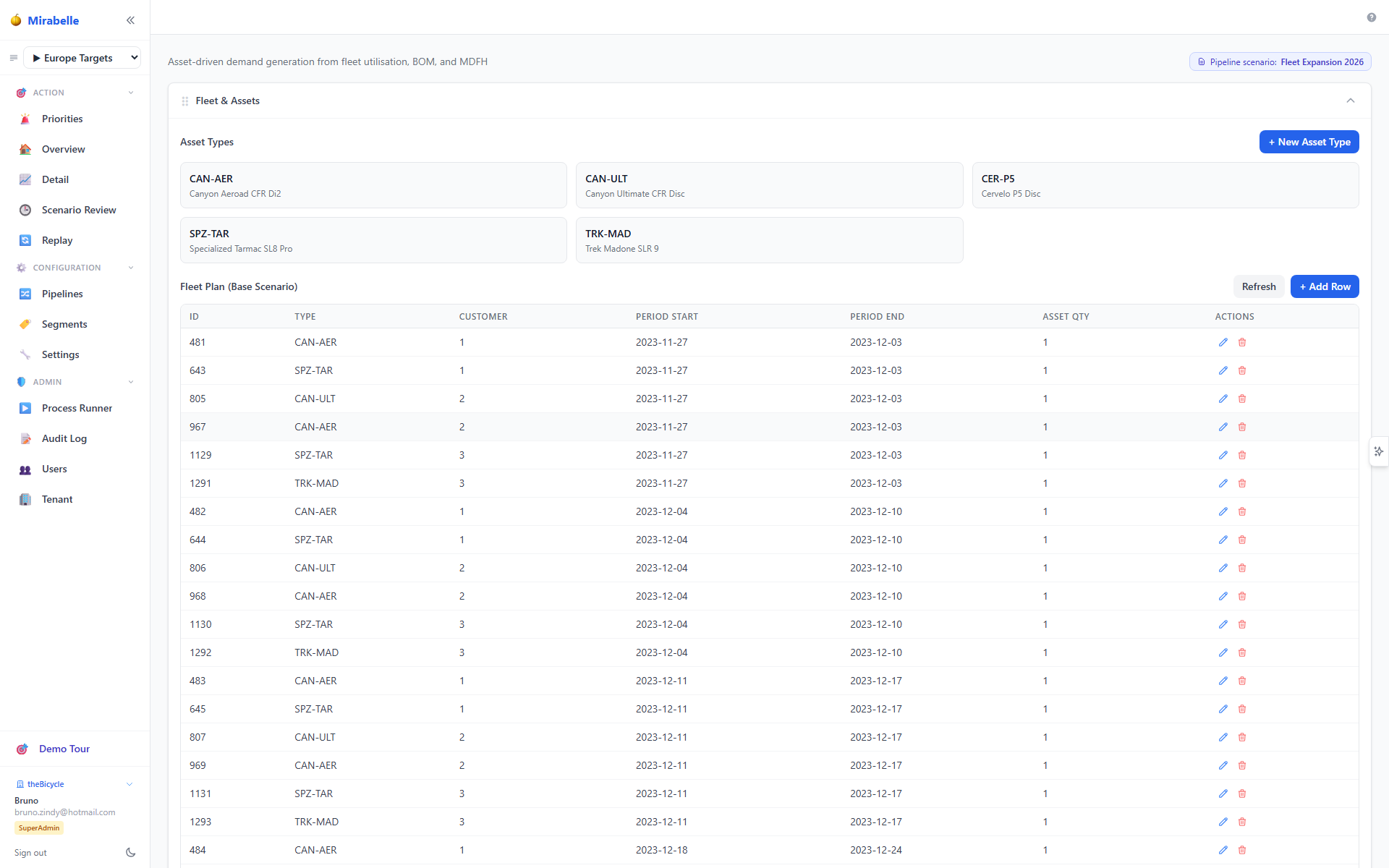
The screen is organised into five draggable, collapsible panels:
Panel 1: Fleet and Assets
This panel shows all asset types and, for the selected asset type, the list of individual assets and their deployments.
Asset Types table — columns: Code, Name. Click a row to select that asset type and populate the Assets sub-table.
Assets sub-table — shows individual assets of the selected type. Click an asset to see its deployment history.
Deployments table — for the selected asset: asset ID, site, start date, end date.
Coverage table — maintenance schedule for the selected asset at each site: event dates, site, and quantity (number of assets covered by the event).
To add a new asset type, click + New Asset Type and fill in the Code and Name.
Panel 2: BOM and Effectivity
Select an asset type from the dropdown to see its causal BOM — the parts consumed during maintenance, with quantities and likelihoods.
The BOM is displayed as both a flat table and an interactive tree (BomExplorer). The tree view shows the hierarchy of sub-assemblies within the asset.
To edit a BOM line, click the edit icon. To add a new part, use the add-row form at the bottom of the table. Save with the Save BOM button.
Panel 3: Scenarios
Causal scenarios allow you to model alternative fleet plans. A base scenario reflects the current plan; alternative scenarios can override fleet sizes, failure rates, or maintenance schedules.
Scenario list columns:
| Column | Description |
|---|---|
| Checkbox | Select one or more scenarios to run |
| Name | Click to open the scenario detail editor |
| Description | Free-text notes |
| Is Base | Whether this is the baseline scenario |
| Granularity | Time grain for the forecast: daily, weekly, monthly, quarterly, or yearly |
| Status | Last run status: running, completed, or error |
To create a new scenario, click + New Scenario. After creation you are taken directly to the scenario editor to set up fleet plan, deployments, usage, failure rates and coverage.
To run one or more scenarios, check their checkboxes and click Run Selected Scenarios. The run is submitted as a background job; status updates automatically.
Panel 4: Results
After running, the Results panel shows the causal demand forecast output. Filter by item and site using the dropdowns.
Results are displayed as a time series chart (one series per scenario) and a table with weekly quantities. You can compare the base scenario against alternatives to quantify the impact of fleet changes or maintenance schedule changes.
The causal forecast for each item-site is also visible in the Time Series Viewer as the amber line labelled "causal".
Panel 5: Customers and Usage
For MRO operations where assets are deployed at customer sites, this panel shows the mapping between customers and their assets, along with usage rate data. Usage data drives the demand calculation alongside failure rates.
Editing a Causal Scenario
Click a scenario name in the Scenarios panel to open the Scenario Detail modal. The modal has six tabs:
All edits are saved automatically — there are no Save buttons. Changes are persisted 800 ms after you stop typing (debounced auto-save). A brief "Saved" confirmation appears in the toolbar when auto-save completes. For new scenarios (no ID yet), the Info tab has a Create & Edit Scenario button; after creation, all subsequent edits auto-save.
Info Tab
Edit the scenario's basic properties:
| Field | Description |
|---|---|
| Name | Scenario label (required) |
| Description | Free-text notes |
| Is Base | Marks this as the baseline scenario |
| Utilisation Multiplier | Slider (0.1–5.0×) that scales fleet utilisation for this scenario. Default 1.0. Use >1 to model increased usage intensity, <1 for reduced operations. |
All fields auto-save when changed (existing scenarios). For new scenarios, fill in the name and click Create & Edit Scenario.
Fleet Plan Tab
View and edit the fleet plan for this scenario — the list of assets and their quantities at each site.
- Granularity — switch between Year / Quarter / Month / Week using the toolbar buttons
- Add row — click the add-row form at the bottom to add a new fleet entry (asset, site, quantity, effective date)
- Edit — click the edit icon on any row to modify quantity or date inline
- Delete — click the delete icon to remove a fleet entry
- Excel navigation — Tab moves to the next cell; Arrow keys navigate cells; Ctrl+C/V copy/paste from Excel
All changes auto-save.
Deployments Tab
View and edit asset-to-site deployment records for this scenario. Each deployment specifies:
| Field | Description |
|---|---|
| Asset | Which physical asset is deployed |
| Site | Where the asset is located |
| Deploy date | When the deployment starts |
| Qty | Number of units at this site |
| Notes | Free-text remarks |
- Add deployment — click + Add Row
- Edit — double-click or type to edit any field inline
- Delete — click the trash icon to remove a deployment
- Excel navigation — Tab = next cell, Ctrl+C/V = copy/paste from Excel
All changes auto-save.
Usage Tab
View and edit asset usage overrides for this scenario. Usage rates determine how intensively each asset is used (e.g. flight hours per month, km per month), which drives the demand calculation.
- Add or edit usage rate entries per customer and usage type
- Overrides are scenario-specific — they don't affect the base scenario or other alternatives
- Excel navigation: Tab, Arrow keys, Ctrl+C/V
All changes auto-save.
Failure Rates Tab
View and edit failure rates for this scenario. Each row specifies:
| Field | Description |
|---|---|
| Item | The spare part / consumable |
| Usage type | Which usage metric drives wear (e.g. km, flight hours) |
| Failure rate | Expected replacements per unit of usage |
| Asset | Optional — override for a specific asset |
| Site | Optional — override for a specific site |
| Position | Optional — override for a specific BOM position |
Failure rates follow the 4-level specificity hierarchy described above. More specific entries override less specific ones.
- Add rate — click + Add Row
- Edit — double-click to modify inline
- Delete — click the trash icon to remove a rate
- Excel navigation — Tab = next cell, Ctrl+C/V = copy/paste from Excel
All changes auto-save.
Coverage Tab
View and edit the maintenance coverage schedule for this scenario. Coverage defines when maintenance events occur and how many assets are covered:
| Field | Description |
|---|---|
| Asset type / Asset | What is being maintained |
| Site | Where the maintenance happens |
| Customer | Optional — customer-specific schedule |
| Coverage % | Percentage of assets covered in the event |
| Valid from / Valid to | Date range for the coverage entry |
- Add coverage — click + Add Row
- Edit — double-click to modify inline
- Delete — click the trash icon to remove a coverage entry
- Excel navigation — Tab = next cell, Ctrl+C/V = copy/paste from Excel
All changes auto-save.
Running Causal Forecasting
- Ensure asset types, assets, and deployments are configured in Panel 1.
- Ensure the BOM is configured in Panel 2 for each asset type.
- Create or select a scenario in Panel 3.
- Select the scenario checkbox and click Run Selected Scenarios.
- Wait for the job to complete (status shown as badge: running → completed or error).
- View results in Panel 4.
Alternatively, causal forecasting runs as part of the full pipeline (forecast step, Phase 5) when the pipeline has a causal_scenario_id configured. Run it from the Process Runner or the Pipelines screen.
Computation Engine
The causal engine runs primarily as a single SQL query on PostgreSQL (the SQL-first path). This is significantly faster than the Python fallback and handles all standard overrides (fleet multipliers, deactivation, retired entries, per-scenario usage replacement). The Python path is only used when a scenario has overrides that SQL cannot express (new fleet entries or per-asset usage patches).
For technical details on the SQL CTE chain, failure rate waterfall, override handling, and parity testing, see the Causal SQL Engine algorithm reference.
How Causal Results Compare to Statistical Methods
Causal forecasting is not always more accurate than statistical methods. It depends on the quality of the input data:
| Condition | Use statistical | Use causal |
|---|---|---|
| Demand history is long and stable | Yes | Maybe |
| Fleet plan is changing (new assets, retirements) | No — statistics cannot see future fleet changes | Yes |
| Demand is driven by scheduled maintenance | No — statistics sees randomness | Yes |
| No reliable deployment or coverage data | Yes | No |
In the Time Series Viewer, the causal forecast appears as a separate line so you can compare it visually against statistical methods and the actuals. The method comparison table shows accuracy metrics for the causal forecast alongside all other methods.
Blended forecasts
You can blend statistical and causal forecasts in the supply netting step. The supply.netting_forecast_type setting (in Settings) controls whether the supply engine uses the statistical forecast, causal forecast, maintenance forecast, or a blend.