Supply Planning
Table of Contents
- Core Concepts
- Route Types
- Supply Projections
- Orders
- BOM Explosion
- Negative On-Hand = Stockout Risk
- Approving Orders from the Exceptions Screen
- Netting
- Supply Planning Scenarios
- Reading the Supply Plan on the Dashboard
- Advanced Supply Planning Features
- Allocation Engine Trigger
Supply Planning is accessible from multiple places:
- The Supply tab within the Time Series Viewer (single series view)
- The Supply Planning tab within the Pipelines screen (scenario management)
- The Dashboard supply plan panel (aggregate view)
Supply planning translates the demand forecast into a week-by-week inventory projection and generates replenishment orders to keep projected on-hand above zero.
Figure: the MRP flow nets multi-source demand, explodes the BOM with pegging, generates planned orders, applies lot-sizing and capacity checks, and firms them into PIPE_supply_orders.
flowchart LR
  DEM["Demand<br/>(stat + maint + causal forecast)"] --> NET["Netting v2<br/>(firm orders, returns)"]
  NET --> EXP["BOM explosion + pegging"]
  EXP --> PO["Planned orders"]
  PO --> LS["Lot-sizing<br/>(min/max/mult)"]
  LS --> CAP["Capacity check<br/>(scheduling.rs)"]
  CAP --> FIRM["Firm / PO<br/>(PIPE_supply_orders)"]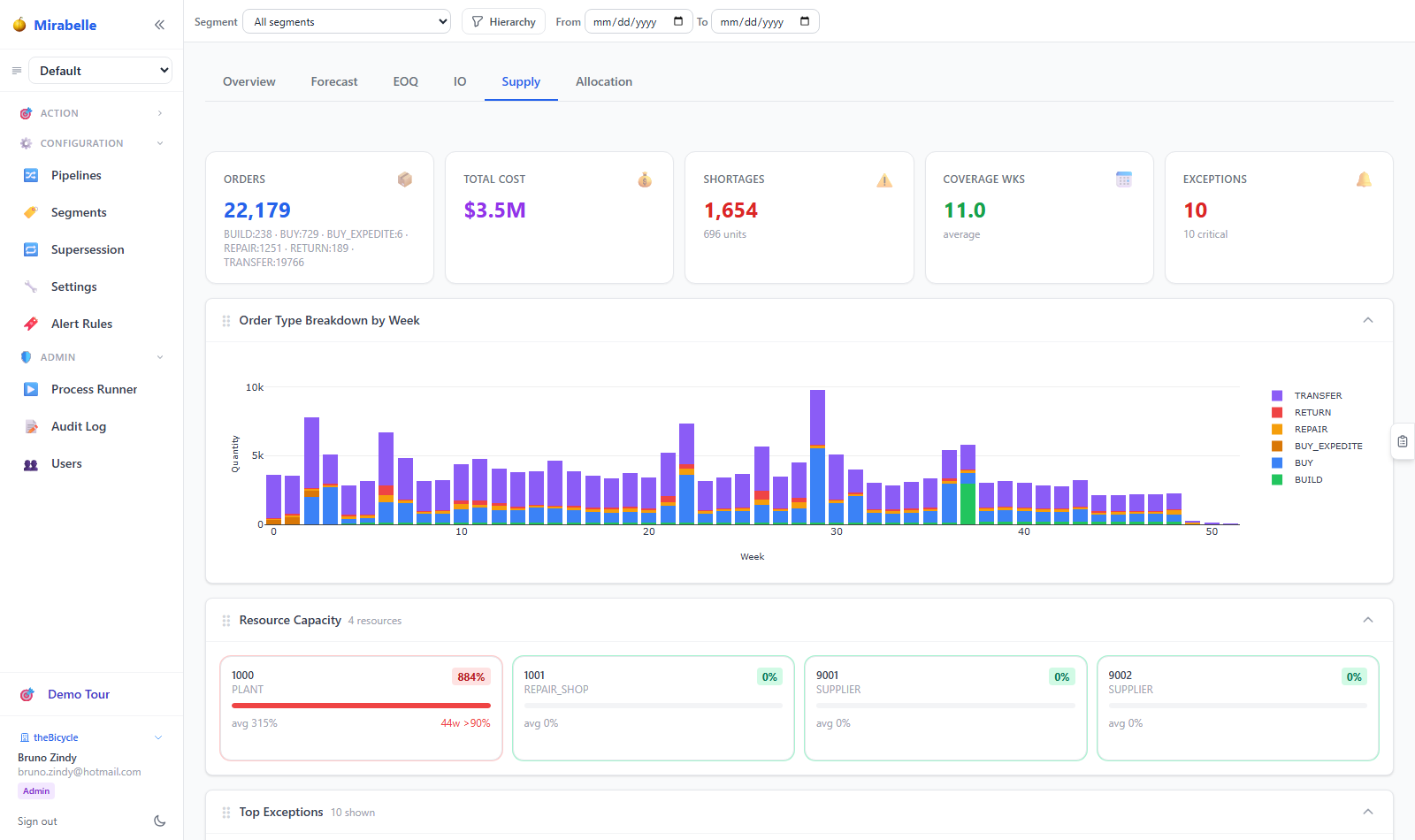
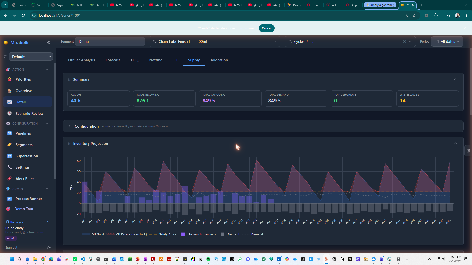
The Supply tab in the Time Series Viewer shows projected on-hand, on-order quantities and expected receipts.
Core Concepts
On-Hand (OH)
On-hand is the physical stock currently in a warehouse or stocking location. In the supply projection, "on-hand" refers to the projected future on-hand — what the model predicts the physical stock will be in each future period, after accounting for expected demand and planned replenishments.
When projected on-hand drops below zero, this represents a stockout: demand is expected to exceed available supply in that period.
On-Order (OO)
On-order is the quantity currently ordered from suppliers or manufacturing, not yet received. On-order stock is expected to arrive and increase on-hand when it lands (on the expected receipt date).
Projected On-Hand
Projected on-hand is calculated week by week:
A week with negative projected OH is a stockout period. These appear as red markers in the supply charts and as Supply exceptions in the Exceptions screen.
Route Types
Mirabelle supports five route types that define how an item is replenished:
| Route Type | Label | Meaning |
|---|---|---|
PURCHASE |
Buy | Order from an external supplier. Creates a purchase order. |
TRANSFER |
Transfer | Move stock from another internal location. Creates a transfer order. |
MAKE |
Build | Manufacture the item internally. Creates a work order. |
RETURN |
Return | Returns from customers create supply. Applies a return rate fraction. |
REPAIR |
Repair | Returned units that can be refurbished. Applies a repair yield fraction. |
A single item can have multiple routes (e.g. primary = PURCHASE, secondary = TRANSFER from another warehouse). The supply engine prioritises routes based on the supply.source_priority configuration: Repair → Return → Transfer → Build → Buy (repair is used first if available).
Lead Times
Each route has a lead time: the number of days between placing the order and receiving the stock. The supply engine uses the route lead time to determine when to place orders:
Lead times can vary over time (historical actuals) and are shown in the Supply Cell sparkline in the Exceptions screen.
Supply Projections
The supply projection is the output of a supply planning run. It shows, for each item-site and each week in the planning horizon:
| Column | Description |
|---|---|
| Period | Week start date |
| Demand Forecast | Netted demand for that week (from the selected forecast type) |
| On-Hand (start) | Projected on-hand at the beginning of the week |
| On-Order | Quantity expected to arrive during the week |
| On-Hand (end) | Projected on-hand at the end of the week, after demand and receipts |
| Safety Stock | The MEIO-recommended safety stock buffer |
| Orders Placed | Any replenishment orders placed in this period |
Weeks where On-Hand (end) is negative are highlighted in red.
Orders
The supply planning engine generates three types of planned orders:
Purchase Orders
Created when an item needs to be bought from a supplier. The order shows:
- Item and site
- Quantity
- Expected order date (when to place the order)
- Expected availability date (when the stock is expected to arrive)
- Supplier route
- Status: planned, suggested, approved
Transfer Orders
Created when stock should be moved from one internal location to another. The order shows source site and destination site in addition to quantity and dates.
Work Orders
The Dashboard Supply tab gives an aggregated view of open orders, shortages and coverage.
Created for manufactured items (MAKE route). Represent internal production orders.
Order Status
| Status | Meaning |
|---|---|
| Planned | System-generated based on the supply projection; no human action yet |
| Suggested | System has recommended this order; waiting for planner approval |
| Approved | Planner has approved; typically means the order will be communicated to the supplier |
Figure: a planned order moves through suggestion to planner approval; edits or rejection return it to the planned pool.
stateDiagram-v2
  [*] --> Planned: system-generated
  Planned --> Suggested: recommended
  Suggested --> Approved: planner approves
  Suggested --> Planned: edited / rejected
  Approved --> [*]
Planners can approve suggested orders directly from the Exceptions screen (Supply Cell) or from the Supply Planning screen.
BOM Explosion
For manufactured items or assemblies, the supply engine performs BOM explosion: the demand for the parent item is propagated down to its component items.
For example, if a finished assembly needs 100 units, and its BOM requires 2 units of Component A and 3 units of Component B, the explosion creates demand of 200 units for Component A and 300 units for Component B. These component demands are added to any direct customer demand for those components.
BOM explosion is handled automatically by the supply planning step. The BomExplorer component in the Time Series Viewer provides a visual tree of any item's BOM structure.
Negative On-Hand = Stockout Risk
Any week where projected on-hand is negative represents a potential stockout. The system surfaces these as:
Figure: a negative projected on-hand triggers the stockout signal, which fans out to UI markers, exceptions, and a likely-cause diagnosis.
flowchart TD
  OH["Projected on-hand[week N]"] --> Q{"< 0?"}
  Q -- "no" --> OK["healthy stock"]
  Q -- "yes" --> ST["Stockout signal"]
  ST --> E1["Red marker on lead-time sparkline"]
  ST --> E2["Supply exception"]
  ST --> E3["Red cell in projection table"]
  ST --> CA{"Likely cause"}
  CA --> C1["safety stock too low"]
  CA --> C2["order delayed / cancelled"]
  CA --> C3["demand spike"]
CA --> C4["lead time increase"]- Red markers on the lead time sparkline in the Supply Cell of the Exceptions screen
- Supply type exceptions in the exception list
- Red cell highlighting in the supply projection table
The on-hand quantity shown (e.g. −34) is the magnitude of the shortfall: 34 units of unmet demand.
The most common causes of projected stockouts:
- Safety stock is too low (MEIO has set insufficient buffer)
- A replenishment order was delayed or cancelled
- Demand spiked above forecast
- A lead time increase means an order will arrive too late
On-Hand at Repair Warehouses
Repair warehouses (sites whose only inbound route type is REPAIR) have a different interpretation of "good stock": because they receive returns and rework them, the useful throughput is the repair output rate rather than a static on-hand balance.
In the supply overview, the OH Bad metric for repair-only sites is calculated from actual REPAIR order quantities rather than from a physical good/bad inventory split. This avoids misleading spikes from units that are in-process rather than truly bad stock.
Approving Orders from the Exceptions Screen
From the Exceptions Supply Cell:
- The next planned order is shown with its ID, quantity, and expected availability date.
- Edit the Qty field if you want to approve a different quantity than planned.
- Edit the Date field if the availability date needs to change.
- Click Approve.
The order status changes to approved. The supply projection does not automatically recalculate at this point — you need to re-run the supply planning step for the projection to reflect the approved order.
Netting
The supply engine does not use the raw statistical forecast directly. It uses a netted forecast that adjusts for:
- Firm orders — known confirmed demand that is more reliable than the forecast
- Return forecast — expected returns from customers, which reduce net demand
- Open purchase orders already placed — these represent supply already committed
- In-transit stock — stock that has been shipped but not yet received
- Multi-source demand — statistical, maintenance, and causal forecasts are combined according to their configured netting modes before consumption logic is applied
The forecast type used for base netting (supply.netting_forecast_type) can be:
- statistical — use the statistical forecast from the forecasting pipeline
- causal — use the causal forecast (if causal forecasting has been run)
- maintenance — use the maintenance/event-driven forecast
- blended — use a weighted combination
The netted forecast is visible in the Netting tab of the Time Series Viewer.
Netting Version
The current supply planning pipeline runs Netting v2 (2026-06). This version introduced safety-stock-aware carry-forward in the Rust engine, multi-source demand handling, two-step netting sequences, parallel computation, ClickHouse-primary persistence, and return forecast projection.
If you are upgrading from an older pipeline version, regenerate the netting table by re-running the supply planning step. The v2 schema adds causal_* columns and changes the netting_direction vocabulary from forward_first / backward_first to forward / backward.
Multi-Source Demand
The netting engine now consumes three independent demand sources:
| Source | Description |
|---|---|
| Statistical forecast | The baseline forecast produced by the statistical forecasting pipeline |
| Maintenance forecast | Event-driven or maintenance-driven demand (e.g. scheduled service parts) |
| Causal forecast | Causal model output (e.g. promotions, weather, external regressors) |
Each source is passed into the netting engine with its own quantity per week. The engine applies the configured netting mode (see below) to each source before computing final net demand.
Netting Modes (add vs net)
For maintenance and causal forecasts, the pipeline configuration (netting_mode_maintenance, netting_mode_causal) can be set to:
| Mode | Behaviour |
|---|---|
add |
The forecast is added to the soft (statistical) forecast. The combined quantity is then consumed by firm orders during netting. |
net |
The forecast is treated as firm-like demand that consumes the soft forecast first. Any remaining soft forecast after net-mode demands are applied is then available for firm customer orders. |
add mode is appropriate when the forecast source represents incremental demand that should be merged with the statistical baseline. net mode is appropriate when the forecast source represents high-certainty demand (e.g. a signed promotion) that should take priority over the statistical forecast.
Two-Step Netting Sequence
When netting_sequence = 'two_step' and at least one of maintenance or causal is configured in net mode, the engine performs netting in two passes:
- First pass —
net-mode demands (maintenance and/or causal) are netted against the soft (statistical) forecast. The soft forecast is consumed forward or backward by these demands, producing a pre-netted remainder. - Second pass — Firm customer orders are netted against the pre-netted remainder (not the original soft forecast). This gives
net-mode forecast demands priority over firm customer orders.
When netting_sequence = 'single' (or no sources are in net mode), all demands are combined into a single soft forecast and firm orders consume that total in one pass.
The netting direction (whether firm orders consume from future forecast periods forward or backward) is controlled by the direction key in the forecast parameter set's netting section: forward or backward.
Safety-Stock-Aware Carry Forward
In the Rust netting engine (files/supply/src/netting.rs), projected on-hand is carried forward week by week using:
where available = previous_carry + supply and demand is the net demand for the period. Previously, whenever available < required (with required = demand + safety_stock), the carry was set to 0.0. This caused false zero-inventory signals and phantom shortages in downstream periods. The v2 engine preserves physical inventory even when the safety-stock buffer is violated, and only reports a shortage when physical stock itself would go negative.
A small epsilon (NETTING_EPS = 1e-4) is used internally to prevent floating-point rounding drift.
Parallel Computation
When more than 50 series are processed in a single netting run, the Python layer parallelises series-level computation via a ThreadPoolExecutor with up to min(cpu_count, 16) workers. Smaller runs remain single-threaded to avoid executor overhead.
Return Forecast Projection
Projected returns are computed from demand (including maintenance forecast when it is in add mode), time-shifted by return_lt_weeks and scaled by return_rate (taken from RETURN routes). The return forecast reduces net demand before the supply engine plans replenishment orders.
Netting Columns
The netting table stores the following per-week quantities:
| Column | Description |
|---|---|
stat_forecast_qty |
Raw statistical forecast |
return_forecast_qty |
Expected return quantity (reduces net demand) |
maint_forecast_qty |
Maintenance-driven forecast quantity |
causal_forecast_qty |
Causal forecast quantity |
firm_demand_qty |
Confirmed firm orders |
total_netted_qty |
Final net demand sent to the supply engine |
stat_netted_qty |
Stat portion after netting |
return_netted_qty |
Return portion after netting |
maint_netted_qty |
Maintenance portion after netting |
causal_netted_qty |
Causal portion after netting |
return_consumed_qty |
Returns that consumed firm demand |
causal_consumed_qty |
Causal demand that consumed the soft forecast |
consumption_enabled |
Whether demand consumption logic is active |
netting_direction |
forward or backward |
is_past |
1 for historical rows, 0 for future. The supply engine only reads is_past = 0 rows. |
Historical rows in netting
PIPE_forecast_netting stores both past and future rows. The supply engine always filters AND is_past = 0. If you query the netting table directly, add this filter to avoid treating historical demand as future demand.
ClickHouse-primary persistence
Starting with v2, PIPE_forecast_netting is persisted to ClickHouse as the primary store. The pipeline uses drop_ch_partition followed by bulk_insert_ch for full-table refresh. Querying the netting table should target the ClickHouse instance.
Supply Planning Scenarios
Like forecasting, supply planning supports multiple scenarios. Different supply scenarios can use:
- Different forecast scenarios as input
- Different MEIO results (safety stock levels)
- Different lead time assumptions
- Different source priority rules
This allows planners to run "what-if" analyses: "what would our inventory projection look like if lead times increased by 2 weeks?" or "what is the impact of switching from a 95% to a 98% service level target?"
Reading the Supply Plan on the Dashboard
The Dashboard's Supply Plan panel (at the bottom, lazy-loaded) shows an aggregate view of the supply projection across all items in the active pipeline. Key KPIs shown:
- Total projected on-hand value
- Total on-order value
- Number of weeks with any stockout (negative OH) events
-
Service coverage: percentage of future demand-weeks covered without stockout
- Allocation Engine Trigger
Advanced Supply Planning Features
Beyond the core projection and ordering logic described above, Mirabelle offers several advanced capabilities that extend the supply planning workflow:
| Feature | Description |
|---|---|
| Capacity & Resource Network | Model production capacities and resource constraints to ensure the supply plan respects real-world throughput limits. See Supply Advanced → Capacity & Resource Network. |
| Calendar Closure Handling | Account for warehouse and plant closures (holidays, maintenance windows) so that orders are not placed on non-working days. See Supply Advanced → Calendar Closure. |
| Sales Returns | Incorporate customer return forecasts as a supply source, reducing net demand and improving on-hand projections. See Supply Advanced → Sales Returns. |
| Demand Profile Builder | Define custom demand profiles (seasonality patterns, growth curves) that override or supplement the statistical forecast for specific item-site combinations. See Supply Advanced → Demand Profile Builder. |
| Consumption Preview | Preview how demand will be consumed by firm orders, returns, and other netting adjustments before running the full supply plan. See Supply Advanced → Consumption Preview. |
| Pegging & Traceability | Trace which demand orders each supply order fulfills, and vice versa — full upstream/downstream linkage for audit and root-cause analysis. See Supply Advanced → Pegging & Traceability. |
| Firm Supply Orders | Treat ERP-originated executed/blocked orders as INPUT to the engine. Two new flags (firm_orders_block_horizon, respect_lead_time) tighten how the engine generates recommendations around them. See Firm Supply Orders. |
Allocation Engine Trigger
Once the supply planning run completes and replenishment orders are generated, the Allocation engine is triggered automatically. The allocation step distributes available supply (on-hand + on-order) across competing demand streams according to prioritisation rules defined in the allocation configuration. This ensures that constrained stock is allocated to the highest-priority channels, customers, or regions first.
For details on allocation rules, priority configuration, and the allocation workflow, see Allocation.