Feature Forecasting / Covariates
This page covers how Mirabelle uses external variables (covariates) alongside historical demand to improve forecast accuracy. Covariates are primarily consumed by the TFT (Temporal Fusion Transformer) model, which natively supports static, known-future, and observed-only inputs.
Overview
Traditional time-series forecasting relies solely on historical demand patterns. In practice, demand is influenced by external drivers — promotions, holidays, pricing, weather — that pure autoregressive models cannot see. Feature forecasting bridges this gap by injecting covariates into the forecasting pipeline.
Figure: flow from defining a covariate in the registry to it influencing the forecast.
flowchart TD
  A["Define feature in Feature Registry"] --> B["Upload CSV values (global or series-specific)"]
  B --> C["Reliability scoring per feature-series pair"]
  C --> D["Feature Parameter Set selects features & min reliability"]
  D --> E["Push/upload values to pipeline-scoped store"]
  E --> F["TFT & NeuralForecast consume covariates"]
  F --> G["Forecast + feature importance scores"]
The TFT model is uniquely suited for this because it:
- Accepts static metadata per series (e.g. brand, category)
- Accepts known-future inputs whose values are available at inference time (e.g. planned promotions)
- Accepts observed-only inputs that enrich training but are not needed at inference time (e.g. weather)
- Produces feature importance scores that tell you which covariates actually drive the forecast
Covariates and method selection
Covariates are consumed by TFT and other NeuralForecast models. Statistical methods (AutoARIMA, AutoETS, Croston, etc.) do not use covariates. When method selection picks a statistical method as the winner for a given series, covariates are simply not used for that series. This is by design — the system selects whatever works best per series.
Covariate Types
Mirabelle classifies covariates into three categories based on their temporal availability:
Figure: distinction between the three covariate categories and where each feeds the TFT model.
flowchart LR
  subgraph REGISTRY["Feature registry"]
    S["Static covariates (once per series)"]
    K["Known-future covariates (future_available = true)"]
    O["Observed-only covariates (future_available = false)"]
  end
  S --> T["TFT static input"]
  K --> T
  K --> TI["TFT futr_exog (training + inference)"]
  O --> TH["TFT hist_exog (training only, zero-fill at inference)"]
Static Covariates
Time-invariant attributes that describe a series. They are stored once per series and do not change over time.
| Example | Description |
|---|---|
| Item category | "Electronics", "Apparel" |
| Brand | Brand name or label |
| Location type | "Warehouse", "Store", "Outlet" |
| ABC class | A / B / C classification |
In the feature registry, static covariates are configured as series-specific features. Their values are the same for every date, but they are stored with a unique_id key so the model knows which series they belong to.
Known-Future Covariates
Variables whose future values are known in advance. These are the most impactful covariates because the model can use them both during training and at inference time.
| Example | Description |
|---|---|
| Planned promotions | Binary flag (0/1) or discount depth |
| Calendar events | Holiday indicator, school holidays |
| Scheduled price changes | Future price or price delta |
| Marketing spend | Planned advertising budget per period |
Known-future covariates have the highest impact
Because the model can use known-future values when generating the forecast, they provide the strongest accuracy lift. A promotion calendar is typically the single most valuable covariate you can add.
In the feature registry, known-future covariates are flagged with future_available = true. The NeuralForecast pipeline maps them to the futr_exog input slot.
Observed-Only Covariates
Variables that are only available historically. They improve training quality but cannot be used at inference time because their future values are unknown.
| Example | Description |
|---|---|
| Weather | Temperature, precipitation |
| Competitor pricing | Actual competitor shelf prices |
| Macroeconomic indicators | GDP, CPI (published with a lag) |
| Stockout flags | Whether the item was out of stock |
In the feature registry, observed-only covariates have future_available = false. The NeuralForecast pipeline maps them to the hist_exog input slot.
Missing future values for observed-only covariates
The model handles observed-only covariates by using zero-fill or the training mean for future periods. This is acceptable because the TFT attention mechanism learns to rely on them only during the historical lookback window.
Preparing Covariate Data
Data Format
Covariate values are uploaded as CSV files. The required columns depend on whether the feature is global (same value for all series on a given date) or series-specific (different values per SKU).
Column Requirements
| Column | Required | Description |
|---|---|---|
date |
Yes | ISO format (YYYY-MM-DD). Must align with the pipeline granularity (weekly, daily, or monthly). |
unique_id |
Series features only | Must match the unique_id used in the demand data. |
value |
Yes | Numeric. Can be binary (0/1), continuous, or categorical-encoded. |
Date Coverage Requirements
Known-future features must span the forecast horizon
For a feature flagged as future_available = true, its values must cover both the historical training window and the full future forecast horizon (typically 24 weeks). If future values are missing, the model will fall back to zero-fill for those periods, which degrades accuracy.
Observed-only features only need to cover the historical training window. However, better historical coverage improves the model's ability to learn the relationship between the covariate and demand.
Feature Registry
The Feature Registry is the central catalogue of all defined covariates. It stores metadata about each feature — name, type, granularity, and whether it is forward-looking.
Managing Features via the UI
Navigate to Pipelines → Forecast, click Edit on the scenario you want to configure, then open the Features tab. The Feature Registry panel lets you:
- Create a new feature — click + New Feature, fill in the form
- Edit an existing feature — click the Edit button on any row
- Upload values — click Upload and select a CSV file
- Clear values — removes all stored values for a feature
- Delete a feature — removes the feature and all its values
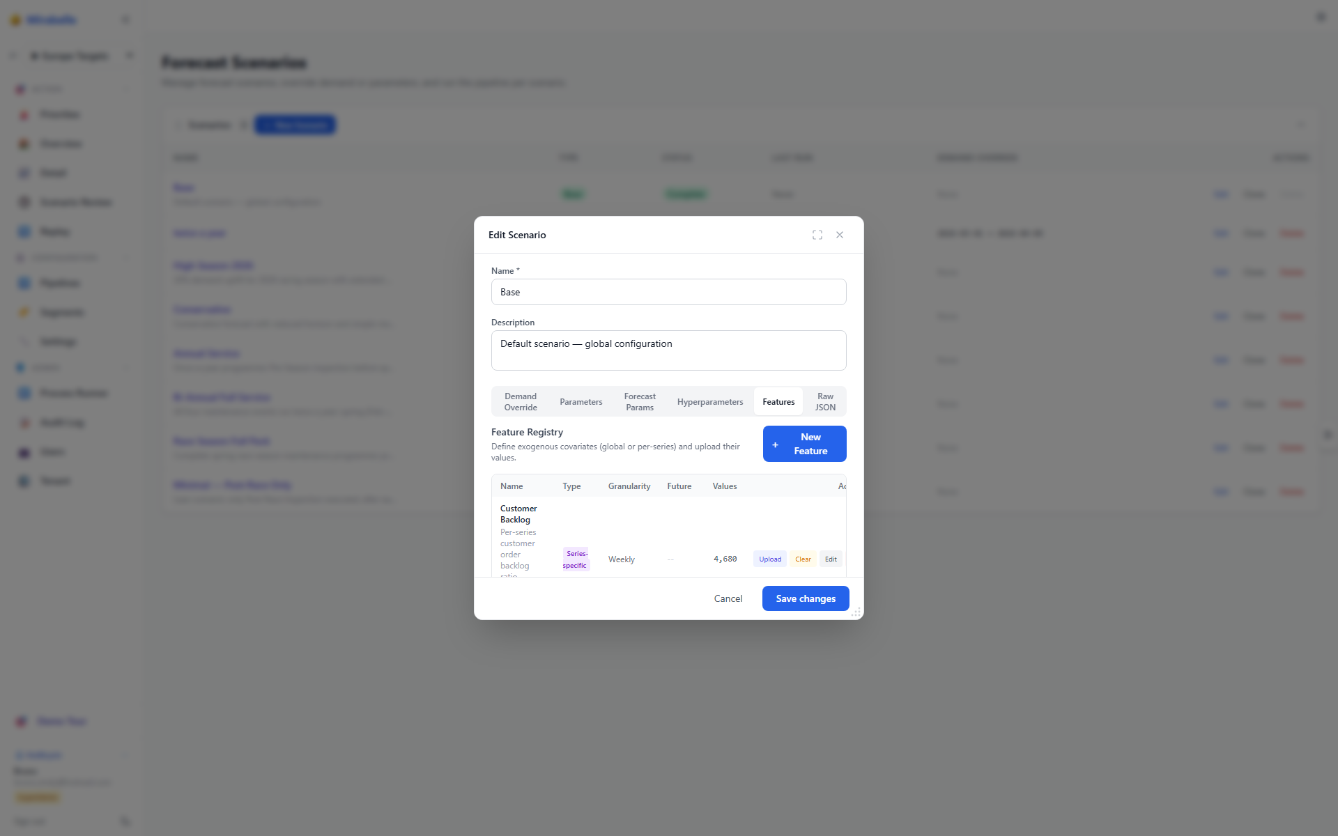
The feature creation form includes:
| Field | Description |
|---|---|
| Name | Unique identifier (e.g. "Holiday Index", "Promo Flag") |
| Description | Optional free-text explanation |
| Type | Global (date only) or Series-specific (date + unique_id) |
| Granularity | Weekly, Daily, or Monthly — must match pipeline frequency |
| Future-available | Toggle on if future values will be known at inference time |
Managing Features via the API
List all features
Returns a list of all registered features with their metadata and value counts.
Create a feature
{
  "name": "Holiday Index",
  "description": "Weekly holiday intensity (0=no holiday, 1=major holiday)",
  "feature_type": "global",
  "future_available": true,
  "granularity": "weekly"
}
Update a feature
Same body schema as create.
Delete a feature
Removes the feature definition and all its stored values.
Feature Value Endpoints
Retrieve feature values
GET /api/features/registry/{feature_id}/values?unique_id=SKU-001&date_from=2026-01-01&date_to=2026-06-30&limit=500
Supports optional filters: unique_id, date_from, date_to, limit.
Upload feature values (CSV)
Upload a CSV file with the column format described in Preparing Covariate Data. Existing rows are upserted — if a value already exists for a given (feature_id, date, unique_id), it is updated.
Clear all feature values
Removes all stored values for the feature but keeps the feature definition.
Feature Values & Reliability
Per-Series Feature Values
When a feature is marked as series-specific, each series (unique_id) has its own value for each date. This is essential for covariates like promotion flags that vary by SKU.
The value upload endpoint handles both global and series-specific features automatically based on the feature's feature_type setting.
Feature Reliability Scoring
Not every covariate improves forecast accuracy. Some may be noisy, sparse, or weakly correlated with demand. The reliability scoring system evaluates each feature–series pair to determine whether the covariate is actually useful.
Same-period vs lagged correlation
A critical distinction in reliability scoring is when a feature correlates with demand:
| Concept | Meaning | Example |
|---|---|---|
| Same-period correlation (lag 0) | Feature value at time t correlates with demand at time t | A price discount and higher demand in the same week |
| Lagged correlation (lag k) | Feature value at time t-k correlates with demand at time t | A promotion in week 1 lifts demand in week 3 (lag 2) |
| Best lag | The lag k at which the absolute correlation is strongest | If best_lag = 2, the feature 2 periods ago predicts current demand best |
The reliability engine computes correlation at every lag from 0 to K and stores the full lag profile — a vector of correlation coefficients, one per lag.
Reliability metrics
| Metric | Description |
|---|---|
| Reliability score | Composite score (0–1) combining correlation, MAPE, and bias |
| Corr (same pd) | Pearson correlation between feature and demand in the same period (lag 0) |
| Best lag | Lag k at which feature[t-k] most strongly correlates with demand[t]; 0 = same period is strongest |
| Best-lag correlation | The signed correlation at the best lag; colored by absolute strength (green ≥ 0.6, amber ≥ 0.4, red < 0.4) |
| Lag profile | Mini bar chart showing correlation at each lag; the best-lag bar is highlighted |
| MAPE | Mean Absolute Percentage Error using the best lag |
| Bias | Systematic over/under-prediction from the feature alone |
| N windows | Number of overlapping observations used |
The scoring engine tests lags up to a frequency-aware default (daily=28, weekly=4, monthly=12, etc.), capped by the available history and the forecast horizon. If a feature has its strongest relationship with demand two weeks later, the reliability score reflects that lagged relationship instead of ignoring it.
Understanding the Lag Profile Chart
Each row in the reliability results table includes a lag profile mini-chart — a small bar chart showing how correlation changes across lags:
Lag profile for a promotion feature (weekly). Lag 2 is highlighted as the best lag — the promotion 2 weeks ago correlates most strongly with current demand (corr = 0.62).
How to read the chart:
- Blue bars = positive correlation (feature and demand move in the same direction)
- Red/pink bars = negative correlation (feature and demand move in opposite directions)
- Bold/darker bar = the best lag — the lag with the strongest absolute correlation
- Lighter bars = other lags, shown for comparison
- The x-axis is the lag number (0 = same period, 1 = one period earlier, 2 = two periods earlier, etc.)
- Hover over any bar to see the exact correlation value
Interpreting common patterns:
| Pattern | What it means | Business implication |
|---|---|---|
| Best lag = 0, all others near zero | Feature affects demand immediately | Price changes, holiday flags |
| Best lag = 1–2, lag 0 weak | Feature has a delayed effect | Promotions with carryover, marketing campaigns |
| Strong negative at lag 0, positive at lag 1 | Feature cannibalises current period, pulls forward from next | Deep discounts that shift demand forward |
| All bars near zero | Feature has no meaningful correlation | Consider removing this feature |
| Alternating positive/negative | May indicate seasonal confounding | Check for overlapping seasonal effects |
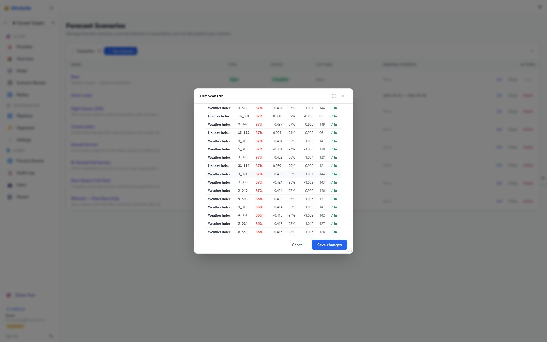
Reliability Results Table Columns
The reliability results panel displays one row per feature–series pair:
| Column | Description |
|---|---|
| Feature | Feature name from the registry |
| Series | unique_id of the demand series |
| Score | Composite reliability score (0–1); colored green ≥ 0.7, amber ≥ 0.4, red < 0.4 |
| Corr (same pd) | Correlation between feature and demand in the same period (lag 0) |
| Best lag | How many periods earlier the feature correlates most strongly with current demand; "0 (same pd)" = same-period correlation is strongest; "N pd earlier" = feature N periods ago is the best predictor |
| Lag profile | Mini bar chart of correlation at each lag (see above) |
| MAPE | Mean Absolute Percentage Error using the best-lag feature shift |
| Bias | Normalised mean signed error |
| N | Number of overlapping observations |
| Gate | Whether the feature passes the minimum reliability threshold (✓ In / ✗ Out) |
A blue info banner above the table summarises the column meanings:
Corr (same pd) = correlation between feature and demand in the same period (lag 0).
Best lag = how many periods earlier the feature correlates most strongly with current demand (e.g. lag 2 means feature 2 periods ago predicts demand today).
Lag profile = correlation at each lag; highlighted bar = best lag (blue = positive, red = negative).
Reliability API
Returns reliability scores per feature–series pair, sorted by score descending. The pipeline_id parameter is required. unique_id is optional.
Response fields:
| Field | Type | Description |
|---|---|---|
feature_id |
int | Registry ID |
feature_name |
str | Feature name |
unique_id |
str | Demand series identifier |
correlation |
float | Same-period (lag 0) Pearson correlation |
best_lag |
int or null | Lag with strongest absolute correlation; 0 = same period |
best_lag_correlation |
float or null | Correlation at the best lag (signed) |
lag_profile |
object | Map of lag → correlation, e.g. {"0": 0.22, "1": 0.14, "2": 0.62, ...} |
mape |
float | MAPE using best-lag feature shift |
bias |
float | Normalised mean signed error |
reliability_score |
float | Composite score (0–1) |
n_windows |
int | Number of overlapping observations |
Example response:
{
  "feature_id": 3,
  "feature_name": "promo_flag",
  "unique_id": "7_305",
  "correlation": 0.22,
  "best_lag": 2,
  "best_lag_correlation": 0.62,
  "lag_profile": {"0": 0.22, "1": 0.14, "2": 0.62, "3": 0.12, "4": -0.08},
  "mape": 0.45,
  "bias": 0.03,
  "reliability_score": 0.68,
  "n_windows": 52
}
Use reliability scores to gate features
The Feature Parameter Sets (see below) support a minimum reliability threshold per feature. Features that score below the threshold for a given series are excluded from that series' forecast, preventing noisy covariates from degrading accuracy.
Customer Forecasts as Features
Customer-submitted forecasts are not a separate data track — they are ordinary features. Each customer's forecast becomes one series-scoped, future-available feature named CF:{customer_code}, and the standard feature-reliability machinery decides whether it is good enough to refine the statistical forecast.
How customer forecasts get in
| Path | Mechanism |
|---|---|
| UI upload | POST /api/customer-forecast/upload (files/api/customer_forecast_router.py) |
| Bulk import | import.customer_forecast staging → the import ETL registers the CF:{code} feature and upserts its values |
| Pipeline aggregate | the customer-forecast-indicator step (files/evaluation/customer_forecast_indicator.py) builds the merged indicator (below) |
Finding the good customers — per-customer reliability
Each CF:{customer_code} feature is scored against that customer's own demand history — this requires customer_id attribution on the master.demand_actuals rows of the series. The evaluator computes the same metrics as any feature (see Feature Reliability Scoring): same-period correlation, lag profile, MAPE, bias, and the composite reliability score.
- Customers scoring below the threshold (parameter
customer_forecast.reliability_min_score, default 0.4) are dropped from the aggregate. - The surviving customers are merged into one aggregate feature,
Customer Forecast, weighted by their reliability scores, with a per-series aggregate reliability row explaining the mix (the qualification modal lists the contributingCF:*customers). - A customer forecast can be systematically mis-scaled yet shape-accurate — high MAPE and large bias with high correlation. The composite score keeps such customers in the aggregate; the consuming model learns the scale.
How a good customer forecast refines the forecast
During the forecast step, the FeatureLoader (files/utils/feature_loader.py):
- resolves the series' feature parameter set (its
external_featureslist +reliability_min_score), - gates each (series, feature) pair by its reliability score — below the gate, the feature is silently excluded,
- aligns the feature to demand at the scored best lag (building lagged variants from the lag profile),
- emits it as training columns for the models.
Which models can actually consume it:
| Family | Methods | Consumption |
|---|---|---|
| Statistical | AutoARIMA, AutoETS, AutoTheta, MSTL, … | Never — univariate only |
| ML tabular | LightGBM, XGBoost | Historical exogenous columns |
| Neural (subset) | NHITS, NBEATS, TFT, DeepAR, PatchTST | Future exogenous (feature must be future_available — CF:* features are) |
| Neural (rest) | MLP, LSTM, RNN, TCN | None |
A customer forecast changes the final number only if a consuming method is enabled in the series' method selection and wins the backtest. If only statistical methods run, the feature is loaded and scored but never used. After a run, check the winning model's feature importance (GET /api/features/series-importance) to confirm the customer forecast actually contributed.
Series uid spellings (import-seeded tenants)
Feature values may be stored under the series' numeric uid (7_5128) or its xuid (GPS55_1000001827) depending on the writer — the import ETL writes xuids, the UI writes numeric. The overlay endpoint and the forecaster's FeatureLoader resolve every spelling of the series (all master.demand_actuals uids naming the same item × site), so a feature scored for a series is also displayed and loaded for it. (Until Aug 2026 both paths were one-way lookups — import-seeded tenants showed empty overlays and silently skipped CF:* features in forecasting.)
Verification checklist — a CF:* feature seems ignored
- Values exist for the series under any uid spelling: check
master_feature_values(loaded_attells you when the upload/indicator last ran). - Demand rows carry
customer_id— without attribution the scorer cannot match the customer to the series and the indicator produces nothing. - Reliability clears the gate: the
pipe_feature_reliabilityrow must meet the param-setreliability_min_score(default 0.4). Click the row to open the qualification modal and inspect score, lag profile, MAPE and bias. - A consuming method is enabled for the series (LightGBM/XGBoost or NHITS/NBEATS/TFT/DeepAR/PatchTST) — otherwise the feature is loaded but unused.
- It won: check feature importance on the winning model.
Reading a reliability row (GPS 2)
CF:1000001827 · score 45% · corr (same pd) 0.909 · best lag 0 (91%) · MAPE 942.9% · bias 10.57 · n = 5
The customer's submitted volumes track the series' shape almost perfectly (corr 0.909 at lag 0, 91% of the lag-profile mass) but are ~10× mis-scaled (MAPE ≈ 943%, bias ≈ 10.6 — the forecast is monthly-lumpy while demand is weekly). The composite score (0.45) still clears the 0.4 gate: the customer stays in the aggregate, and the consuming model learns the scale correction.
Configuring TFT with Covariates
Defining features in the registry is not enough — you must also configure which features the TFT model should use via Feature Parameter Sets.
Temporal Correlation and Lagged Features
A common concern with feature forecasting is whether the model understands that a feature in one period can influence demand in a later period. TFT learns some temporal dependencies implicitly through its attention and recurrent layers, but Mirabelle can now make delayed effects explicit through temporal lags.
How it works
For each feature–series pair, the reliability step computes a cross-correlation profile: the correlation between demand at time t and the feature at times t-k for a range of lags k. The strongest lag is stored as best_lag. Feature parameter sets can then instruct the loader to create additional lagged columns.
Cross-correlation: feature(t−k) vs demand(t)
| Week | Promo flag | Demand | Lag 0 | Lag 1 | Lag 2 ★ | Lag 3 |
|---|---|---|---|---|---|---|
| W1 | 1 | 100 | 1↔100 | — | — | — |
| W2 | 0 | 130 | 0↔130 | 1↔130 | — | — |
| W3 | 0 | 160 | 0↔160 | 0↔160 | 1↔160 | — |
| W4 | 0 | 110 | 0↔110 | 0↔110 | 0↔110 | 1↔110 |
A promotion in W1 (blue cell) lifts demand in W3 (green cell). Lag 0 pairs each week's promo with the same week's demand (low correlation). Lag 2 pairs promo(t−2) with demand(t) — the W1 promo aligns with the W3 demand spike, producing the highest correlation.
| Mode | Behaviour |
|---|---|
auto |
Adds the original feature plus one column shifted by best_lag, if it passes the minimum correlation threshold |
distributed |
Adds columns for every lag from 0 to K |
best_only |
Adds only the column shifted by best_lag |
Lagged columns are named feature_name_lag_k (the contemporaneous column keeps the original name). For future-available features, lagged values are forward-filled from the latest known values.
Configuration
In the scenario editor's Features tab, inside each parameter set, enable the Temporal lags toggle and choose:
- Mode: auto / distributed / best_only
- Max lag K: hard upper bound on the lag; defaults to a frequency-aware value
- Minimum absolute correlation: only lags with
|corr| ≥ thresholdare used inauto/best_onlymodes
Recommended defaults:
| Frequency | Default K | Meaning |
|---|---|---|
| Daily | 28 | ~4 weeks |
| Weekly | 4 | 4 weeks |
| Monthly | 12 | 1 year |
| Quarterly | 4 | 1 year |
| Yearly | 2 | 2 years |
K is automatically capped by the smaller of the default, n_observations / 4, and the forecast horizon.
Pipeline API / JSON schema
The temporal_lags block lives inside each feature parameter set's params:
{
  "features": [1, 3, 5],
  "reliability_min_score": 0.4,
  "temporal_lags": {
    "enabled": true,
    "mode": "auto",
    "max_lag": 4,
    "min_abs_corr": 0.15
  }
}
Which models consume lagged features?
- NeuralForecast models (TFT, NHITS, NBEATS, DeepAR, PatchTST): lagged future-known features are added to
futr_exog_list; historical-only features becomehist_exog_list. - ML models (LightGBM, XGBoost): lagged columns are appended to the engineered feature matrix.
Start with auto mode
auto adds at most one extra column per feature and is the safest way to capture a dominant delayed effect without exploding the feature count.
Feature Parameter Sets
A Feature Parameter Set is a named configuration that specifies:
- Which features from the registry to include
- A minimum reliability score per feature (optional)
- Which segments the parameter set applies to
- Whether temporal lags are enabled for this set
Each scenario can have multiple parameter sets, ordered by priority. The default parameter set applies to all series not covered by a segment-linked set.
Creating Parameter Sets
In the scenario editor's Features tab, below the Feature Registry, you will find the Feature Parameter Sets panel:
- Seed Default — creates the default parameter set (includes all registered features with no minimum reliability)
- Add Set — creates a new named parameter set
- Assign Segments — link the set to one or more segments; series in those segments will use this set instead of the default
- Toggle Features — enable/disable individual features within each set
- Set Minimum Reliability — per feature, set the threshold below which the feature is excluded for that series
- Enable Temporal Lags — choose a lag mode, max lag K, and correlation threshold
Parameter Set API
List parameter sets for a scenario
Returns all parameter sets with their features, segments, and ordering.
Create a parameter set
{
  "name": "Promo-heavy segments",
  "params": {
    "features": [1, 3, 5],
    "reliability_min_score": 0.4
  }
}
Update a parameter set
Same body schema as create.
Assign segments to a parameter set
Reorder parameter sets
Delete a parameter set
Cannot delete the default parameter set
The default set is protected. If you need to remove all features, simply disable them within the set instead.
Seed the default parameter set
Creates the default parameter set with all registered features enabled and reliability_min_score = 0.0. If a default set already exists, this is a no-op.
Pipeline Integration
Feature values must be loaded into the pipeline-scoped ClickHouse store before the forecast step can use them. There are two ways to do this:
1. Push from Registry to Pipeline
If you have already uploaded feature values to the master registry (PostgreSQL), you can push them to a specific pipeline/scenario in ClickHouse:
This copies all values for the given feature from master_feature_values (PG) into PIPE_feature_values (CH). The feature metadata (name, type, future_available) is resolved automatically.
In the UI, the Push Registry → CH button pushes all features at once.
2. Upload Directly to Pipeline
Alternatively, upload a CSV directly into the pipeline-scoped store:
POST /api/features/pipeline/{pipeline_id}/scenario/{scenario_id}/values/upload
Content-Type: multipart/form-data
The CSV must include a feature_name column so the system can resolve it against the registry:
feature_name,date,value,unique_id
holiday_index,2026-01-06,0.0,
promo_flag,2026-01-06,1.0,SKU-001
promo_flag,2026-01-06,0.0,SKU-002
Pipeline-Scoped Feature Values
Retrieve pipeline feature values
Returns feature values stored in ClickHouse for the given pipeline/scenario combination.
Feature summary
Returns aggregated metadata per feature:
| Field | Description |
|---|---|
feature_id |
Registry ID |
feature_name |
Feature name |
feature_type |
global or series |
future_available |
Whether the feature is forward-looking |
global_rows |
Count of rows without a unique_id |
series_rows |
Count of rows with a unique_id |
date_from |
Earliest date with values |
date_to |
Latest date with values |

Clear pipeline feature values
Truncates all feature values from ClickHouse for the pipeline/scenario.
Clearing pipeline values is irreversible
This deletes all feature data from the ClickHouse pipeline store. You will need to re-push or re-upload values before the next forecast run.
Series-Level Analysis
Feature Overlay on Time Series
The feature overlay endpoint returns covariate values aligned with a specific time series, enabling visualization of how features co-vary with demand.
Returns feature values for the given series, grouped by feature:
[
  {
    "feature_id": 1,
    "feature_name": "holiday_index",
    "feature_type": "global",
    "dates": ["2026-01-06", "2026-01-13", "..."],
    "values": [0.0, 1.0, "..."]
  }
]
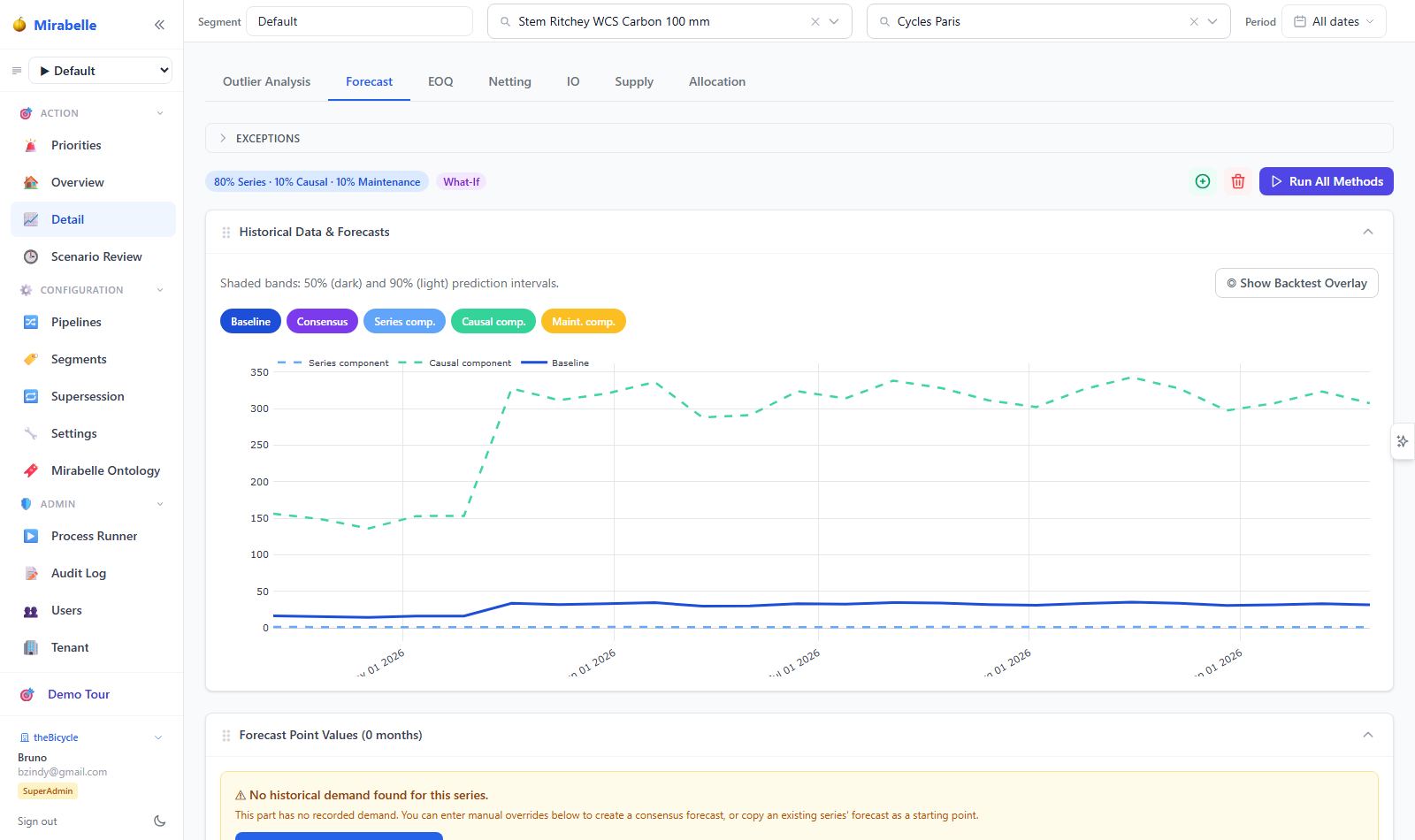
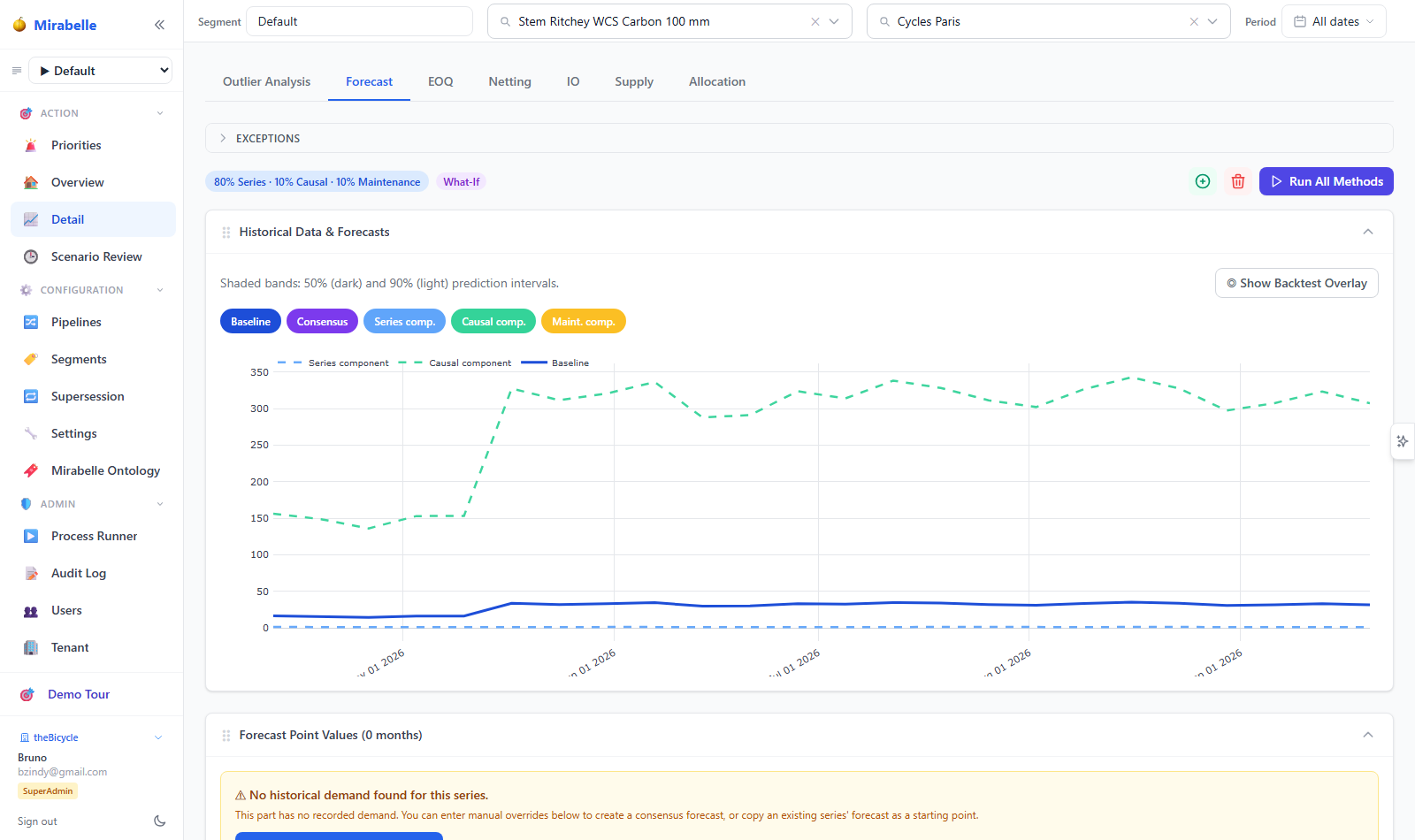
This data powers the Features overlay in the Time Series Viewer, where covariates are rendered as dotted traces on a secondary axis on top of the demand chart, and can be toggled per feature with the FEATURES chips.
Series values may be stored under the series' numeric uid or its xuid (import-seeded tenants) — the endpoint resolves every uid spelling of the series (all master.demand_actuals uids naming the same item × site), so both writers' values appear.
Clicking a feature chip's ⓘ button — or a row in the Feature Reliability panel — opens the Feature Qualification Modal: a feature-vs-demand dual-axis chart (with a best-lag alignment toggle), the reliability metrics (score, correlations, lag profile, MAPE, bias), and the winning model's feature-importance share; for the Customer Forecast aggregate it also lists the contributing per-customer CF:* scores.
Feature Importance Ranking
The TFT model produces per-series feature importance scores as a byproduct of its attention mechanism. These scores tell you which covariates the model actually relied on for each series.
Returns importance scores normalised to sum to 1.0, sorted descending:
[
  { "feature_name": "promo_flag",      "importance": 0.42 },
  { "feature_name": "holiday_index",   "importance": 0.31 },
  { "feature_name": "weather_index",   "importance": 0.15 },
  { "feature_name": "brand_category",  "importance": 0.12 }
]
How TFT Uses Feature Importance
The Temporal Fusion Transformer uses a multi-head attention mechanism that learns variable selection weights during training. At a high level:
- Static covariates are fed into a variable selection network that produces context vectors
- Known-future and observed-only covariates pass through time-varying selection weights
- The attention heads learn which features to attend to at each time step
- After training, the aggregated attention weights serve as the importance scores
Features with very low importance (< 0.05) are effectively ignored by the model. You can use this feedback to simplify your covariate set — remove consistently unimportant features to reduce noise and computation time.
Best Practices
Start Small
3–5 well-understood covariates beat 50 noisy ones
Begin with a small set of covariates you understand well — typically a promotion flag, a holiday index, and a price variable. Add more only if they show meaningful reliability scores and feature importance. TFT's variable selection can ignore unhelpful features, but a large feature set increases the risk of overfitting and slows training.
Prioritise Known-Future Covariates
Known-future covariates (promotions, price changes, calendar events) have the most impact because the model can use them at both training and inference time. Observed-only covariates (weather, competitor pricing) provide a smaller marginal improvement since their future values are not available during forecasting.
Validate Feature Reliability Before Pushing to Pipeline
Before pushing features to a pipeline, check their reliability scores. A feature with a reliability score below 0.3–0.4 for most series is likely adding more noise than signal. Use the minimum reliability threshold in Feature Parameter Sets to automatically gate out weak features.
Ensure Consistent Coverage
TFT handles missing values gracefully (zero-fill), but consistent coverage improves accuracy. Gaps in known-future covariates are particularly harmful because the model interprets missing future values as "no event" — if you have a promotion planned but forgot to upload the flag, the model will not account for it.
| Covariate type | Required coverage | Impact of gaps |
|---|---|---|
| Known-future | Historical + full horizon | High — missing future values cause under-forecasting |
| Observed-only | Historical window | Moderate — model falls back to mean |
| Static | Per series (any date) | Low — constant across time |
Check Feature Importance After Runs
After a pipeline run with covariates enabled, review the feature importance scores. If a covariate consistently scores below 0.05 across most series, consider removing it. This reduces model complexity and training time without sacrificing accuracy.
Align Granularity
Ensure the feature granularity matches the pipeline frequency. A weekly pipeline expects weekly feature values. If you have daily data, aggregate it to weekly before uploading. Mismatched granularity causes alignment issues during the forecast step.
Demo Features
For testing and exploration, you can seed demo features:
This creates three sample features — Holiday Index, Weather Index, and Customer Backlog — with synthetic values, in both PostgreSQL and ClickHouse. Safe to call multiple times (uses upsert semantics).