Advanced Supply Planning¶

This page covers the advanced supply planning features of Mirabelle — capacity modelling, demand profiling, returns management, calendar closures, consumption preview, scenarios, pegging, and planning horizon configuration.

For the fundamentals of supply projections, route types, and order management, see Supply Planning.

Table of Contents¶

Supply Capacity & Resource Network
Resource Constraints & Constraint Algebra
Demand Profile Builder
Sales Returns
Calendar Closure
Consumption Preview
Supply Scenarios
Pegging & Traceability
Planning Horizon

Supply Capacity & Resource Network¶

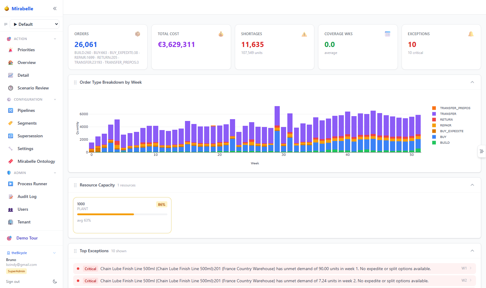
Capacity constraints model the finite production, storage, or shipping limits of your resources. When a resource is fully utilised, the supply engine cannot schedule additional orders through it — even if demand exists — resulting in constrained or delayed orders.

Supply Capacity

Capacity Constraints per Resource/Site¶

Each resource (a machine, a warehouse bay, a shipping lane) has a weekly capacity quantity — the maximum units it can handle. The supply engine tracks both the available capacity and the used quantity per week:

Field	Description
`resource_type`	Category of resource (e.g. `machine`, `dock`, `line`)
`resource_id`	Unique identifier within the resource type
`week`	Planning week index (0–51)
`capacity_qty`	Maximum throughput for this week
`used_qty`	Quantity already committed by planned orders
`utilisation`	Ratio `used_qty / capacity_qty` (0–1)

Overloaded resources

When utilisation exceeds 90%, the resource is flagged as overloaded. When it exceeds 60%, it is tight. Overloaded resources cause the supply engine to defer or constrain downstream orders.

Resource Items¶

A resource is linked to items via the route → route_resource relationship. The resource-items endpoint resolves which items consume a given resource's capacity and by how much:

Field	Description
`item_id`	Item that uses this resource
`item_name`	Display name
`site_name`	Location where the resource is consumed
`route_type`	Which replenishment route uses this resource
`qty_per_unit`	Capacity consumed per unit of item produced/shipped

Use this to understand which items will be affected when a resource is constrained.

Resource Network Graph¶

The resource network endpoint returns nodes (locations) and edges (source → destination lanes) that a resource is involved in. This enables a graph visualisation of your supply network:

Component	Description
Nodes	Unique locations (warehouses, plants) that either send or receive via this resource
Edges	Route lanes showing `from_site → to_site`, the route type, and item count

Figure: the resource network is a graph of location nodes connected by route-lane edges, with the shared resource constraining the lanes it serves.

flowchart LR
  subgraph N["Nodes (locations)"]
    W1["Warehouse A"]
    W2["Warehouse B"]
    P1["Plant C"]
  end
  W1 ==TRANSFER==> P1
  P1 ==MAKE==> W2
  W2 ==BUY==> SUP["Supplier"]
  RES["Resource<br/>(machine / dock / line)"] -.constrains.-> P1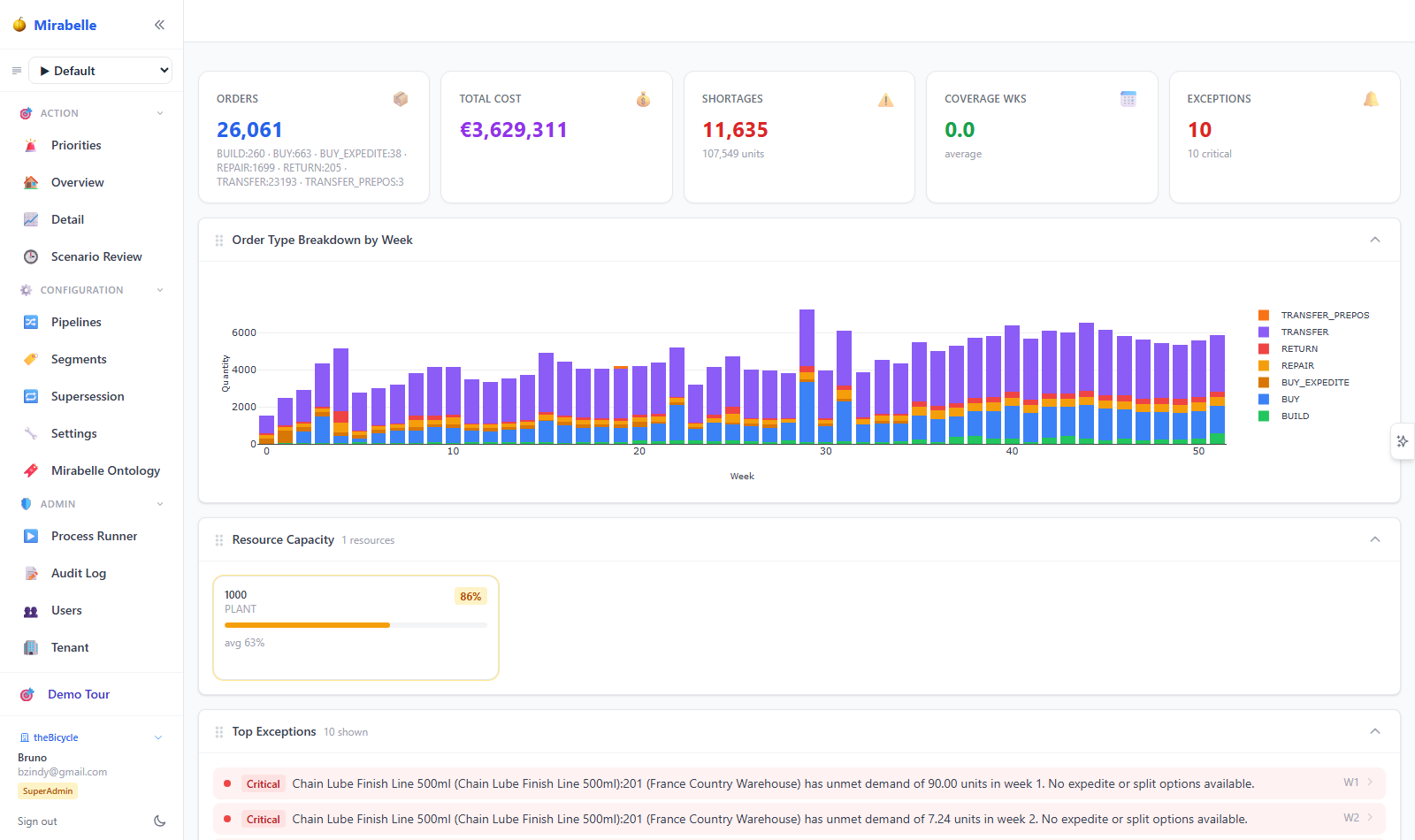

Resource Network

API Reference¶

Capacity UsageResource ItemsResource Network

GET /api/supply/capacity

Parameter	Type	Required	Description
`pipeline_id`	int	No	Filter to pipeline
`scenario_id`	int	No	Filter to scenario
`resource_type`	str	No	Filter to a specific resource category

Returns an array of {resource_type, resource_id, week, capacity_qty, used_qty, utilisation}.

GET /api/supply/capacity/resource-items

Parameter	Type	Required	Description
`resource_type`	str	Yes	Category of resource
`resource_id`	str	Yes	Resource identifier
`pipeline_id`	int	No	Filter to pipeline

Returns items linked to this resource through routes.

GET /api/supply/capacity/resource-network

Parameter	Type	Required	Description
`resource_type`	str	Yes	Category of resource
`resource_id`	str	Yes	Resource identifier

Returns {resource_type, resource_id, nodes: [...], edges: [...]}.

Resource Constraints & Constraint Algebra¶

Beyond the basic capacity model described above, Mirabelle provides a rich constraint algebra that models how real-world limits — lane throughput, warehouse space, machine capacity, production rates — affect supply planning. Constraints operate on two levels:

Capacity scheduler (production) — the existing scheduling.rs module that enforces per-resource weekly limits and pushes orders forward when capacity is full.
Constrained solver (advanced) — the newer solver.rs module that supports soft/hard constraint modes, ranked alternatives (delay, premium transport, overtime, subcontract), and full explanation traces.

Constraint Kinds¶

Constraint Kind	What It Bounds	Where It Applies	Status
LaneCapacity	Max flow volume per week on a transport lane (A → B)	Route (shipping lane between two locations)	Active in constrained solver
LocationStock	Max & min stock level at a location, plus holding and overflow costs	Location (warehouse, plant)	Struct defined — not yet evaluated by solver
ResourceCapacity	Hard capacity + soft overtime band per week	Resource (machine, line, repair centre)	Active in both scheduler and solver
ProductionRate	Per-item production rate on a specific resource	Resource × Item	Struct defined — not yet evaluated by solver
CampaignBatch	Batch minimums, changeover costs	Campaign / batch	Stub — reserved for future

Hard vs Soft Constraints¶

Every constraint can operate in one of two modes:

Mode	Behaviour	When to Use
Hard	Violation is forbidden. The solver must find an alternative (delay, premium transport, subcontract). If no alternative exists, the order is marked `Constrained`.	Regulatory limits, physical impossibilities (a warehouse literally cannot hold more than X units)
Soft	Violation is allowed at a cost. The solver compares alternatives and picks the cheapest feasible plan.	Preferential limits, overtime capacity, premium freight — where exceeding the limit is expensive but not impossible

Figure: a constraint branches by mode — hard violations force an alternative (or mark the order Constrained), while soft violations incur a cost function and the solver picks the cheapest feasible plan.

flowchart TD
  C["Constraint<br/>(LaneCapacity / ResourceCapacity / ...)"] --> M{"mode"}
  M -- "hard" --> HA["violation forbidden"]
  HA --> ALT{"alternative exists?"}
  ALT -- "yes" --> AL["delay / premium / subcontract"]
  ALT -- "no" --> CON["order = Constrained<br/>(CapacityExceeded)"]
  M -- "soft" --> SO["violation allowed at cost"]
  SO --> CF{"cost function"}
  CF -- "linear" --> CL["cost_per_unit x overflow"]
  CF -- "fixed" --> CF2["fixed_cost"]
  CF -- "step" --> CS["piecewise tiers"]
  SO --> PK["pick cheapest feasible plan"]

Violation Cost Functions (Soft Mode)¶

When a soft constraint is exceeded, the violation cost is calculated using one of three cost functions:

Cost Function	Formula	Use Case
Linear per unit	`cost = cost_per_unit × overflow_qty`	Simple overtime premium (e.g. €5 per unit above capacity)
Fixed	`cost = fixed_cost` (independent of overflow magnitude)	A flat penalty for any breach (e.g. €500 changeover fee)
Step function	Piecewise linear: each threshold bucket has its own rate	Tiered pricing — first 10 overflow units at €2/u, next 50 at €5/u, above that at €8/u

Modelling Constraints on a Route¶

Route-level constraints are modelled through the route → resource relationship:

Define the resource in master.supply_capacity with its weekly capacity_qty and used_qty.
Link the route to the resource via master.route_resource, which specifies:
resource_id — which resource constrains this route
resource_type — category (e.g. machine, dock, line)
qty_per_unit — capacity consumed per unit of item produced/shipped
Set the constraint mode in the supply parameters:
soft_capacity_multiplier (default 1.2) — orders up to hard × multiplier use the soft (overtime) band
overtime_cost_multiplier (default 1.5) — cost factor for overtime capacity usage
Set soft_capacity_multiplier = 0 to enforce hard capacity only (no overtime band)

When the supply engine runs, it:

Builds a capacity map: (resource_id, week) → remaining_capacity
For each constrained order, tries to place it at its release week
If insufficient capacity → checks the soft (overtime) band
If soft band is also exceeded → pushes the order to the next available week
If no slot in the entire horizon → marks the order as Constrained and creates a CapacityExceeded exception

Modelling Constraints on a Node / Location¶

Location-level stock constraints (LocationStock) define:

Field	Description
`location_id`	The warehouse or plant
`max_qty`	Maximum stock level (overflow triggers cost)
`min_qty`	Minimum stock level (below this is a service risk)
`holding_cost_per_unit_per_week`	Normal holding cost within limits
`overflow_cost_per_unit_per_week`	Extra cost per unit per week when stock exceeds `max_qty`

These constraints are defined in the constraint algebra (constraints.rs) but are not yet wired into the production solver. They are planned for a future release that will add warehouse-space-aware planning.

Where to Review Applicable Constraints¶

Surface	What It Shows	How to Access
Supply Capacity tab	Per-resource weekly capacity, used, utilisation %, status (overloaded / tight / available)	Supply Planning → Capacity tab
Resource Network	Graph of locations and lane edges for a resource	`GET /api/supply/capacity/resource-network`
SKU Flow	Full constraint analysis for one SKU×site: exceptions + routes with resource status + constrained orders	`GET /api/supply/sku-flow`
Exceptions screen	`CapacityExceeded` severity=Critical exceptions	Exceptions screen → filter by Supply type
Orders grid	Orders with status `Delayed`, `Constrained`, or `Overtime`	Supply Planning → Orders tab → filter by status
Resource Items	Which items consume a resource, and `qty_per_unit`	`GET /api/supply/capacity/resource-items`

How to Know a Constraint Applied¶

There are three signals a planner can observe:

1. Order Status Badge¶

Order Status	Badge Colour	Meaning
Planned	Green	Normal — no constraint triggered
Overtime	Orange	Order used the soft capacity band (overtime cost applies)
Delayed	Amber	Order was pushed to a later week because the resource was fully booked at its preferred week
Constrained	Red	No capacity slot found in the entire horizon — this order cannot be fulfilled

2. Exception Record¶

When a resource is fully exhausted across all weeks, a CapacityExceeded exception is generated with:

severity = Critical
exception_type = CapacityExceeded
The qty that could not be scheduled
A message identifying the resource and the item/site affected

These appear in the Exceptions screen (Supply type filter) and in PIPE_supply_exceptions (ClickHouse).

3. Capacity Utilisation¶

The capacity panel shows three status levels:

Status	Condition	Meaning
Available	Peak utilisation ≤ 60%	Resource has spare capacity
Tight	60% < Peak utilisation ≤ 90%	Resource is approaching its limit
Overloaded	Peak utilisation > 90%	Resource is at or above capacity — downstream orders are being affected

Modelling a Supplier Closing for a Month Every Year¶

A recurring supplier closure is best modelled as a Calendar Closure assigned to the BUY route(s) that source from that supplier. This leverages the existing calendar pull-forward logic, which automatically pre-positions inventory before the closure.

Step-by-Step Setup¶

Create a calendar in Settings → Master Data → Calendars:
Name: e.g. "Supplier X Annual Shutdown July 2027"
Type: working
Mode: not_available — the dates you enter are the closed periods
Description: optional — e.g. "Supplier factory closes for annual maintenance"
Add the closure date range:
Click + Add Entry
From: first day of the closure (e.g. 2027-07-01)
To: last day of the closure (e.g. 2027-07-31)
Label: e.g. "Annual maintenance shutdown"
Click Save entries

The year view will immediately highlight the closed weeks in red.

Assign the calendar to the BUY route via SQL (route management UI is planned):

-- Find the calendar id
SELECT id FROM master.calendar WHERE name = 'Supplier X Annual Shutdown 2027';

-- Find the BUY route sourcing from this supplier
SELECT r.id, i.name AS item, ls.name AS source_supplier, ld.name AS dest_site, r.lead_time
FROM   master.route r
JOIN   master.route_type rt ON rt.id = r.type_id
JOIN   master.item         i  ON i.id  = r.item_id
JOIN   master.location     ld ON ld.id = r.site_id
LEFT   JOIN master.location ls ON ls.id = r.source_site_id
WHERE  rt.planning_type = 'BUY'
ORDER  BY r.id;

-- Assign the calendar
UPDATE master.route
SET    ship_calendar_id = <calendar_id>
WHERE  id = <route_id>;

Re-run supply planning. The engine will automatically:
Convert date ranges to week indices
Identify closed weeks on the source site
Pull demand forward: accumulate demand from closed weeks into a single pre-position order in the last available week before the closure
Tag the order as TRANSFER_PREPOS (or equivalent _PREPOS suffix) so planners can distinguish it from regular replenishment
Set demand to zero during closed weeks — the pre-positioned stock covers them

What the Inventory Projection Shows¶

Week | Opening | Incoming         | Demand | Closing
  18 |   40    | 20 (Buy)         |  20    |   40
  19 |   40    | 100 (Pre-Pos)    |  20    |  120   <- large pre-position delivery
  20 |  120    |  0               |  20    |  100   |
  21 |  100    |  0               |  20    |   80   |  closure weeks —
  22 |   80    |  0               |  20    |   60   |  drawing down
  23 |   60    |  0               |  20    |   40   |  pre-positioned stock
  24 |   40    | 20 (Buy)         |  20    |   40   <- normal resumes

No red cells in weeks 20-23 — the pre-positioned stock covers all demand during the closure. If demand was higher than forecast, shortages will appear in the later closed weeks.

Alternative: Seasonal Capacity Reduction¶

If the supplier doesn't fully close but instead reduces capacity (e.g. runs at 30% during August), model this as a capacity constraint with reduced capacity_qty for the affected weeks in master.supply_capacity. The scheduling engine will push orders to weeks where more capacity is available, but won't generate pre-position orders automatically.

API Reference¶

SKU Flow (Constraint Analysis)

GET /api/supply/sku-flow

Parameter	Type	Required	Description
`item_id`	int	Yes	Item
`site_id`	int	Yes	Site
`pipeline_id`	int	No	Filter to pipeline
`scenario_id`	int	No	Filter to scenario

Returns {item_id, site_id, exceptions, routes, constrained_orders} where each route includes its linked resources with weekly utilisation data and status (overloaded / tight / available).

Demand Profile Builder¶

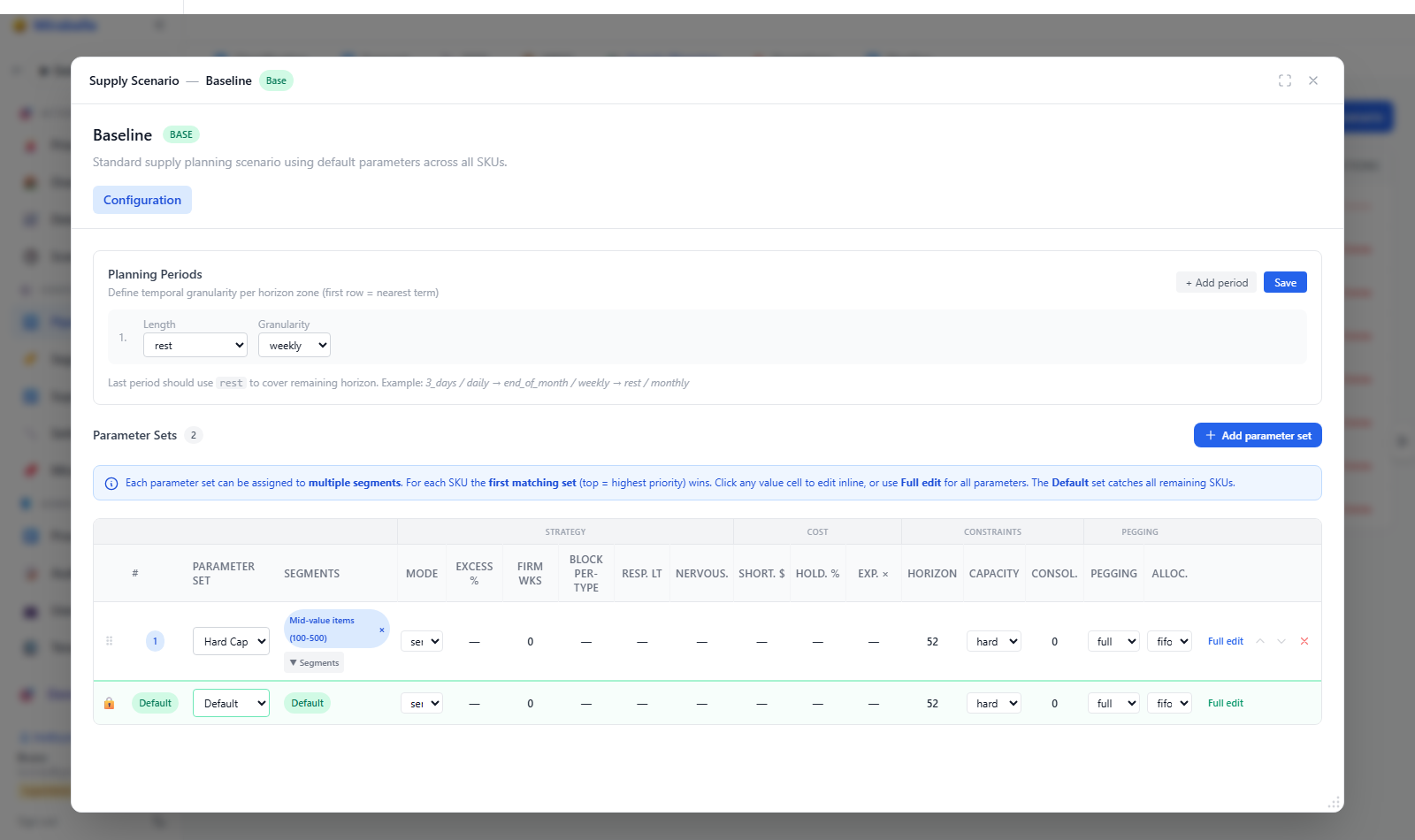
Demand profiles capture the shape of demand within a planning period — how demand distributes across days of the week or sub-weeks. The supply engine uses these profiles to disaggregate weekly or monthly forecast totals into finer-grained supply buckets.

Demand Profile

How Profiles Work¶

For each item × site pair, the builder analyses historical demand patterns and produces a set of weights that sum to 1.0. When the supply engine needs to split a weekly forecast of 100 units across 7 days, the profile determines that, for example:

Monday: 18% (18 units)
Tuesday: 14% (14 units)
Wednesday: 16% (16 units)
...
Sunday: 8% (8 units)

This matters when lead times or calendar closures create partial-week receiving windows.

Granularity Options¶

Granularity	Description
`daily`	Day-of-week (DOW) weights — 7 weights per profile
`weekly`	Trivial single-bucket — stored for completeness, used when no sub-week detail is needed

Lookback Window¶

The lookback_weeks parameter controls how much historical data is used to compute the weights. The default is 26 weeks (6 months). Longer lookback windows produce smoother profiles; shorter windows are more responsive to recent pattern changes.

Choose lookback wisely

Use a 26-week lookback for items with stable weekly patterns. Use a shorter window (8–12 weeks) for items whose demand shape shifts with seasonality (e.g. weekend-heavy in summer, weekday-heavy in winter).

API Reference¶

Build ProfilesGet Profile

POST /api/supply/demand-profile/build

Parameter	Type	Required	Description
`pipeline_id`	int	Yes	Pipeline to build profiles for
`granularity`	str	No	`daily` (default) or `weekly`
`lookback_weeks`	int	No	Historical window (4–104, default 26)

Returns {status, profiles_written, pipeline_id, granularity}.

GET /api/supply/demand-profile

Parameter	Type	Required	Description
`pipeline_id`	int	Yes	Pipeline
`item_id`	int	Yes	Item
`site_id`	int	Yes	Site
`granularity`	str	No	`daily` (default) or `weekly`

Returns {pipeline_id, item_id, site_id, granularity, weights: [...]}.

Sales Returns¶

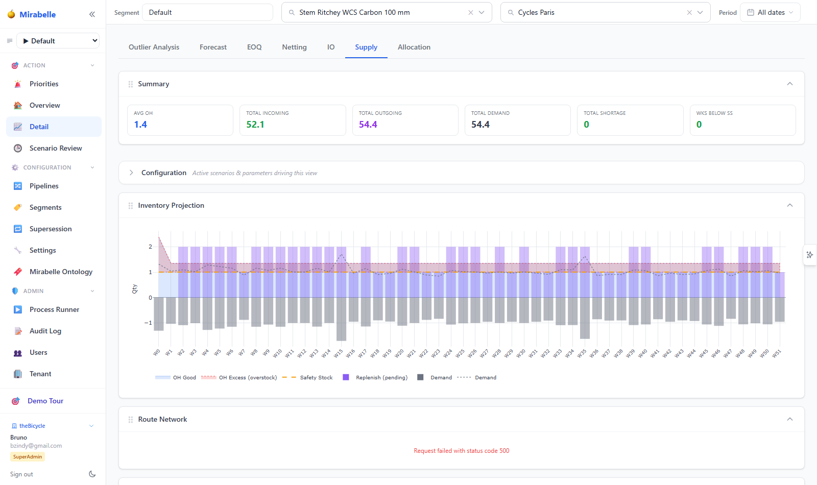
Sales returns model the flow of product back from customers into your inventory. They are distinct from the statistical return rate modelled on RETURN-type routes — sales returns represent known, confirmed, or anticipated return events.

Sales Returns

Return Flow in the Supply Engine¶

Returns reduce net demand: if a customer is expected to return 50 units in week 12, the supply engine treats that as 50 units of incoming supply, reducing the quantity it needs to order. The engine nets confirmed/anticipated returns against the statistical return forecast, so you don't double-count.

Return Statuses¶

Status	Meaning
`anticipated`	Expected based on historical patterns; not yet confirmed
`confirmed`	Customer has confirmed the return; quantity and date are firm
`received`	Product has been physically received back into inventory
`cancelled`	Return was expected but has been cancelled

Only returns with status anticipated or confirmed are factored into supply projections. received returns have already been absorbed into on-hand. cancelled returns are excluded.

Return Entry Fields¶

Field	Description
`item_id`	Item being returned
`site_id`	Location receiving the return
`return_date`	Expected receipt date (ISO `YYYY-MM-DD`)
`qty`	Quantity being returned
`scenario_id`	Which supply scenario this return belongs to
`customer_ref`	Optional reference to the customer or RMA number
`notes`	Free-text notes

API Reference¶

List ReturnsCreate ReturnUpdate ReturnDelete Return

GET /api/supply/sales-returns

Parameter	Type	Required	Description
`item_id`	int	No	Filter by item
`site_id`	int	No	Filter by site
`scenario_id`	int	No	Filter by scenario
`status`	str	No	Filter by status

POST /api/supply/sales-returns

Body: {item_id, site_id, return_date, qty, scenario_id, status?, customer_ref?, notes?}

PUT /api/supply/sales-returns/{return_id}

Body: same fields as create.

DELETE /api/supply/sales-returns/{return_id}

Calendar Closure¶

Calendar closures define periods when a site (typically a source warehouse or plant) is not available for shipping. The supply engine uses this information to pre-position inventory before closures, avoiding stockouts during shut-down periods.

Calendar Closure

How Closures Affect Supply Planning¶

When the supply engine encounters a route whose source site has a calendar closure in a future week, it:

Identifies closed weeks — weeks where the shipping calendar marks the source site as unavailable.
Pulls demand forward — accumulates the demand that would have been ordered during closed weeks and places a single pre-position order in the last available week before the closure.
Tags the order as TRANSFER_PREPOS (or the equivalent route type with a _PREPOS suffix) so planners can distinguish it from regular replenishment.
Sets demand to zero in closed weeks — the pre-positioned stock covers those weeks instead.

Calendar Modes¶

Mode	Meaning
`not_available`	The dates listed are the closed periods; all other dates are open
`available`	The dates listed are the open periods; all other dates are closed

The default and most common mode is not_available — you list the holidays and shutdowns.

Calendar Entry Structure¶

Each calendar entry is a date range:

Field	Description
`date_from`	First day of the closed (or open) period
`date_to`	Last day of the closed (or open) period
`label`	Human-readable label (e.g. "Annual Maintenance Shutdown")

Pre-Position Order Sizing¶

The pre-position quantity equals the total demand across all closed weeks. For example, if weekly demand is 80 units and the site is closed for weeks 20–23:

Week 19: order = 80 (own demand) + 80×4 (closed weeks) = 400 units
Weeks 20–23: demand = 0 (covered by pre-positioned stock)

The destination site draws down from pre-positioned stock each week — no shortage occurs.

Impact on Inventory Projection¶

During closed weeks, the inventory projection will show:

Zero supply received at the destination (no shipments from the closed source)
Declining on-hand as demand consumes the pre-positioned stock
No shortage if the pre-position quantity was sufficient

If the pre-positioned stock is not enough (e.g. demand was higher than forecast), shortages will appear in the later closed weeks.

Assigning Calendars to Routes¶

Calendars are assigned at the route level via the ship_calendar_id field on master.route. Only routes with a calendar assigned will trigger the pre-positioning logic.

API Reference¶

List CalendarsGet CalendarCreate CalendarUpdate CalendarUpdate EntriesDelete Calendar

GET /api/calendars

Parameter	Type	Required	Description
`type`	str	No	Filter by calendar type

Returns calendars with id, name, type, mode, description, entry_count.

GET /api/calendars/{calendar_id}

Returns the calendar header plus its full entries array.

POST /api/calendars

Body: {name, type, mode, description, entries: [{date_from, date_to, label}, ...]}

PUT /api/calendars/{calendar_id}

Updates calendar header fields.

PUT /api/calendars/{calendar_id}/entries

Replaces all entries for a calendar.

DELETE /api/calendars/{calendar_id}

Consumption Preview¶

The consumption preview shows how demand will consume supply before committing to a plan. It computes the netting of firm orders against the raw forecast and the netting of confirmed returns against the statistical return forecast — for a single item × site — without running the full supply engine.

Consumption Preview

What It Shows¶

The preview returns 52-week arrays for both the demand side and the return side:

Demand side:

Array	Description
`raw_forecast`	The statistical forecast before netting
`firm_orders`	Confirmed customer orders by week
`net_demand`	Forecast after firm orders have consumed (netted) into it

Return side:

Array	Description
`statistical`	Return forecast derived from the route's `return_rate × repair_yield`
`confirmed`	Sales returns with status `confirmed` or `anticipated`
`net_returns`	Return forecast after confirmed returns have consumed into it

Netting parameters are also returned so you can understand the logic applied:

Parameter	Description
`forward_fence`	How many weeks forward a firm order can consume from the forecast
`backward_fence`	How many weeks backward a firm order can consume
`direction`	`forward_first` or `backward_first`
`forecast_type`	Which forecast type is used for netting

When to Use It¶

Before a supply run — preview how netting will shape the demand input
When firm orders change — see the impact of adding or removing confirmed orders
When return expectations change — verify that confirmed returns net correctly against the statistical return forecast
Debugging netting parameters — compare forward_first vs backward_first to choose the right direction

API Reference¶

GET /api/supply/consumption-preview

Parameter	Type	Required	Description
`item_id`	int	Yes	Item
`site_id`	int	Yes	Site
`pipeline_id`	int	Yes	Pipeline
`scenario_id`	int	Yes	Scenario

Returns {item_id, site_id, pipeline_id, scenario_id, weeks, demand, returns, netting_params}.

Supply Scenarios¶

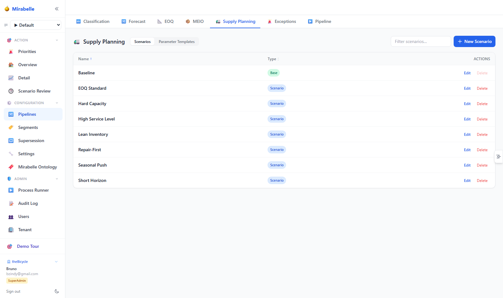
Supply scenarios allow what-if planning by varying supply parameters without modifying the base plan. Each scenario has its own parameter set, its own order outputs, and its own inventory projections.

Supply Scenarios

Scenario Structure¶

Field	Description
`name`	Scenario name (e.g. "Long Lead Time — +2 weeks")
`description`	Free-text description
`parameter_id`	Default parameter set to use
`is_base`	Whether this is the read-only Default scenario
`param_overrides`	JSON dict of parameter overrides merged on top of `parameter_id` defaults
`created_by`	User who created the scenario

Parameter Overrides¶

Instead of creating an entirely new parameter set for each scenario, you can specify overrides — a JSON dictionary of parameter key-value pairs that are merged on top of the base parameter_id. For example:

{
  "lead_time_weeks": 5,
  "safety_stock_multiplier": 1.2
}

This means "use all default parameters, but override lead time to 5 weeks and increase safety stock by 20%".

Segment-Level Parameters¶

Scenarios support per-segment parameter overrides. Each segment (see Segments) can be assigned a different parameter set within the same scenario. The supply engine resolves parameters per item-site by checking:

Segment-level parameter (if the item-site belongs to a segment with an override)
Scenario-level param_overrides (merged on top of the segment parameter)
Scenario's default parameter_id (fallback)

The segment priority order is configurable via sort_order.

Base Scenario¶

The Default (is_base = true) scenario is read-only — it cannot be renamed, modified, or deleted. This protects the production plan from accidental changes.

API Reference¶

List ScenariosCreate ScenarioGet ScenarioUpdate ScenarioUpdate Param OverridesDelete ScenarioGet Segment OverridesSet Segment Overrides

GET /api/supply/scenarios

Returns all scenarios ordered by is_base DESC, created_at ASC.

POST /api/supply/scenarios

Body: {name, description?, parameter_id?, is_base?, param_overrides?}

GET /api/supply/scenarios/{scenario_id}

PUT /api/supply/scenarios/{scenario_id}

Body: {name?, description?, parameter_id?, param_overrides?}

Base scenario is read-only

Updating the base scenario returns HTTP 400.

PUT /api/supply/scenarios/{scenario_id}/param-overrides

Body: {param_overrides: {...}}

Replaces the full override dict.

DELETE /api/supply/scenarios/{scenario_id}

Requires admin role. Base scenario cannot be deleted.

GET /api/supply/scenarios/{scenario_id}/segments

Returns the ordered segment → parameter mapping.

PUT /api/supply/scenarios/{scenario_id}/segments

Body: {overrides: [{segment_id, parameter_id, sort_order}, ...]}

Full replace — the supply order in the array determines priority.

Pegging & Traceability¶

Pegging links each supply order to the specific demand it fulfills. This provides full traceability: for any order, you can answer "which customer demand weeks does this order cover?" and, conversely, "which orders are satisfying the demand in week N?"

Figure: the planner queries pegging two ways — by order (full upstream chain) and by demand week (which orders cover a shortage) — both resolved against PIPE_supply_orders.

sequenceDiagram
  participant U as Planner
  participant A as API
  participant S as Supply engine
  participant DB as PIPE_supply_orders
  U->>A: GET /api/supply/pegging/{order_id}?full_chain=true
  A->>S: resolve pegging tree
  S->>DB: query order + children + demand week
  DB-->>S: pegging rows
  S-->>A: root, children, demand_week, total_cost
  A-->>U: pegging tree (upstream chain)
  U->>A: GET /api/supply/pegging?week=N
  A->>S: demand-side pegging
  S-->>A: demands pegged to week N
  A-->>U: demands + min_week + max_week

Pegging

Pegging Concepts¶

Term	Definition
Demand week	The planning week whose demand is being satisfied
Supply week	The week the supply order is scheduled to arrive
Pegging record	A link between an order and a demand week, with the quantity pegged

Pegging Tree¶

For a single supply order, the pegging tree shows:

The root order — its type, item, site, arrival/release weeks, quantity, and cost
Children — downstream demand entries or sub-orders that this order feeds
The demand week — which demand week(s) the root order satisfies
The total cost of the pegged chain

Use full_chain=true to trace the entire upstream supply chain from raw materials to finished goods.

Demand-Side Pegging¶

The demand-side pegging endpoint returns all supply orders pegged to a given demand week. This answers: "If I have a shortage in week 14, which orders were supposed to cover it?"

It also returns min_week and max_week so the UI can render a week selector with the correct range.

API Reference¶

Demand Pegging (by week)Pegging Tree (by order)Order Pegging (legacy)

GET /api/supply/pegging

Parameter	Type	Required	Description
`week`	int	Yes	Demand week to query
`pipeline_id`	int	No	Filter to pipeline
`scenario_id`	int	No	Filter to scenario
`item_id`	int	No	Filter by item
`site_id`	int	No	Filter by site

Returns {demands: [...], min_week, max_week}.

GET /api/supply/pegging/{order_id}

Parameter	Type	Required	Description
`order_id`	int	Yes	Supply order ID
`full_chain`	bool	No	Include full upstream chain
`pipeline_id`	int	No	Filter to pipeline
`scenario_id`	int	No	Filter to scenario

Returns {root, rows, demand_week, total_cost}.

GET /api/supply/orders/{order_id}/pegging

Returns {order, pegging} — the order details plus its flat pegging list.

Order ID must be positive

Orders generated by the supply engine without a persistent database ID (id=0) cannot be pegged. The API returns HTTP 404 for order_id ≤ 0.

Planning Horizon¶

The planning horizon defines how far into the future the supply engine plans and how time is bucketed. By default, Mirabelle uses a 52-week horizon with weekly buckets. Advanced configurations can use varying granularity — for example, daily buckets for the first 4 weeks and weekly buckets for the remaining 48.

Planning Horizon

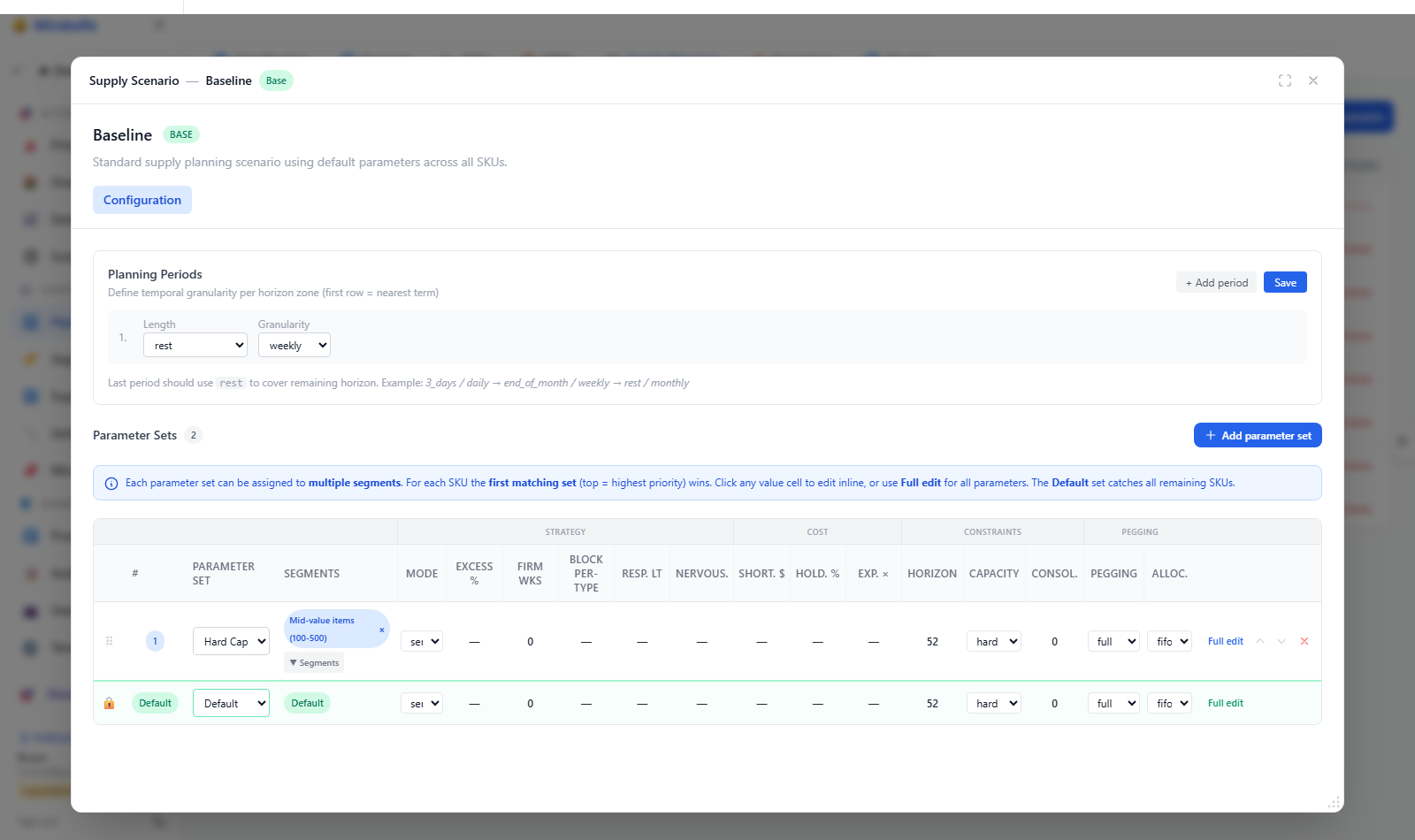
Planning Periods¶

The planning_periods configuration (stored in the scenario's param_overrides) defines the bucket structure. Each period specifies:

Property	Description
`granularity`	`daily` or `weekly`
`duration`	Number of days/weeks in this period
`count`	How many consecutive buckets of this granularity

Example configuration:

{
  "planning_periods": [
    {"granularity": "daily",  "duration": 1, "count": 28},
    {"granularity": "weekly", "duration": 1, "count": 24}
  ]
}

This creates 28 daily buckets (4 weeks) followed by 24 weekly buckets, for a total of 52 buckets spanning 52 weeks.

Horizon Response¶

The planning horizon endpoint returns:

Field	Description
`horizon_start`	ISO date of the first bucket
`planning_periods`	Parsed period definitions
`bucket_count`	Total number of planning buckets
`buckets`	Array of bucket descriptors (first 20 for preview)

Each bucket descriptor:

Field	Description
`idx`	Bucket index (0-based)
`start`	ISO start date
`end`	ISO end date
`granularity`	`daily` or `weekly`
`iso_week`	ISO week number
`days`	Number of days in the bucket

API Reference¶

GET /api/supply/planning-horizon

Parameter	Type	Required	Description
`pipeline_id`	int	Yes	Pipeline to query
`granularity`	str	No	`weekly` (default) or `daily`

Returns {pipeline_id, horizon_start, planning_periods, bucket_count, buckets}.

Horizon and demand profiles

The planning horizon configuration interacts with the Demand Profile Builder. When the horizon uses daily buckets, the supply engine uses DOW-weight profiles to distribute weekly forecast totals across days within each bucket.